Posts tagged “programming”
- Calcolare le differenze dei valori di una serie e ottenere una nuova sequenza.
- Ripetere l’operazione finché tutti i nuovi valori sono zero.
- Aggiungere uno zero extra e ricostruire i valori precedenti con la stessa regola.
- Part 1: $x - p = c$ quindi $x = p + c$, dove $p$ e $c$ sono gli ultimi numeri della riga precedente ($p$) e quella corrente ($c$).
- Part 2: $p - x = c$, quindi $x = p - c$. Qui $p$ e $c$ sono i primi valori della precedente/corrente.
- Ho costruito le combinazioni di due interi che sommano al valore del tempo totale della gara. Ho moltiplicato i due interi per ottenere la distanza.
- Ho selezionato solo quelle combinazioni la cui distanza era maggiore del valore riportato nell’input.
- Ho contato le combinazioni rimaste.
- Singolo
@è uno shortcut per[___]:f[a]coincide conf@a. - Doppio
@@è sinonimo diApply - Triplo
@@@è sinonimo diMapApply, una combinazione diMap(scorciatoia/@) eApplydi cui sopra. È talmente comune questa operazione che si merita un simbolo a parte. - Anche nel nostro input, l’intervallo di cui fare lo scan non è enorme. È grande, ma ancora gestibile. Un codice scritto in Python impiega forse un paio di secondi. Forse con un linguaggio compilato impiegherebbe anche meno.
- Sfruttiamo la matematica: possiamo ricavare gli estremi dell’intervallo in cui cadono le soluzioni, e poi approssimarne gli estremi agli interi più vicini. Ci basta poi fare la differenza di questi due estremi per ottenere le soluzioni. Questa seconda strada è praticamente istantanea.
-
Verificare se un numero $N$ è coperto da questa regola. In questo esempio, controlliamo se $0 \leq (N - 101) < 4$.
-
Se non è coperto, si passa alla regola successiva, se ce n’è una. Se questa è l’unica regola, fine: si restituisce il valore.
-
Se è coperto da questa regola, dobbiamo scoprire dove finisce. In questo esempio: $(N - 101) + 13$.
- Il primo numero vincente che possediamo vale 1.
- Dal secondo numero in poi in nostro possesso, il punteggio raddoppia.
- I numeri vincenti per ogni carta
- Quali copie ricevo per ogni carta
-
C’è una funzione che userò talmente tante volte che ne ho definita una scorciatoia:
SplitLines[s]non è built-in, ma è un alias diStringSplit[s, "\n"]. ↩︎ - Scorro l’input riga per riga, tenendo traccia dell’indice di riga1.
- In ogni riga, estraggo le cifre numeriche e le loro posizioni, che saranno anche le coordinate lungo l’asse delle colonne.
- Con l’indice di riga a portata di mano, costruisco le posizioni
{i, j}sulla griglia che corrispondono alle singole cifre di ogni numero incontrato. Esempio dalla griglia riportata sopra: 467 ha indici colonna da 1 a 3, più l’indice di riga 1. Le posizioni di cui controllare i vicini saranno:{{1, 1}, {1, 2}, {1, 3}}. - Se almeno una delle posizioni occupate dalle cifre di un numero contengono un simbolo nelle posizioni adiacenti, allora il numero è valido.
- Alla fine, si sommano tutti i numeri validi.
- La mia lista di numeri validi ne include alcuni che non lo possono essere perché, per esempio, circondati solo da punti.
- Alcuni numeri vengono contati più del necessario. Come faccio a saperlo? Ho eliminato dal mio set di numeri quelli sicuramente corretti, e ho calcolato la somma dei restanti. Se i numeri fossero contati tutti correttamente, questa somma deve coincidere con la differenza dei totali dei due set. Cioè:
-
Gli indici degli array in Wolfram partono da 1, non da 0. È una scelta coerente con uno degli aspetti più profondi del linguaggio, magari ne discuterò più avanti. ↩︎
-
Il constraint scritto come una
Associationdiventa<| 'red' -> 12, 'green' -> 13, 'blue' -> 14 |>. ↩︎ - The
StringCases[..., x: DigitCharacter :> ToExpression@x]is doing the extraction part: any digit character (0-9) is converted into an expression – that is, an integer, in this case. The result will be a list in which each element contains the digits found on a certain row. #[[{1, -1}]]& /* FromDigits /@it’s a single function mapped onto the list of lists obtained above. The symbol/*is the right composition operator. It means that its right operand will be applied on the result obtained after applying its left operand.#[[{1, -1}]]&takes the first and last elements. If it’s a single item list, it takes the element twice.FromDigitsconstructs an integer from the list of its decimal digits.- The last bit is the map operator
/@.
- Lastly, we compute the total of the reconstructed numbers.
- Find the positions (
{start, end}) of the digits 0-9, either as a number or in letters. - Extracts all portions of the string that correspond to the positions found in step 1.
- At this point, it can apply
numberRulesand convert everything to numeric digits.ToExpressiondoes the same thing as before: it normalizes strings representing numbers into integers. -
By
dayNI will henceforth denote the raw input of a given day, as it can be downloaded from Advent of Code website. ↩︎ - It falls straight down until it meets the first obstacle, whether sand or rock.
- If it cannot occupy the lowest slot directly along its falling path, it slides left and then down (thus
-x → +y). - If the slot on the left is not available either, it slides to the right (
+x → +y). -
I found the numeric answers to the puzzle, but by disassembling and reassembling someone else’s solution written in the Wolfram Language. If I don’t get to the solution by my own conceptual and implementation efforts, then it counts for very little. The two stars have no gusto. ↩︎
- If they are integers, the order is the usual one: smaller numbers will come first. In the first case of the example, 1 vs. 1 is not decisive, but 3 vs. 5 is obvious.
- If both elements are lists, we compare their elements one by one. If the first list contains an integer greater than its corresponding one in the second list, then the order of the packets is wrong. If the first list contains fewer elements than the second, the order is correct (and will be incorrect vice versa). If the order cannot be determined, we must continue with the next part of the input.
- If only one of the two elements is an integer and the other is a list, we must convert the integer to a list (like
1 → [1]) and retry the comparison. -
Alas, graphs are a subject about which I know almost nothing. I left aside the problem of Day 12 as a “holidays assignment.” I will study more and come back with the solution in due time. ↩︎
-
From the official documentation of Python. ↩︎
-
Or use
itertools.chain, which I discovered today. So much can be learned! ↩︎ -
A small bonus, useful as a future reference. Here is the CPython implementation of the
itertools.cmp_to_keyfunction. Another tidbit to keep in mind. ↩︎ -
You can try it at this website. Copy and paste the pattern and input shown just above. Select “Python” in the “Flavor” menu on the left. ↩︎
-
As we read the input, each monkey is a dictionary to which corresponds a
countkey that is initialized to 0. ↩︎ -
It’s quite straightforward. If
A mod p1 ≠ 0but(A mod P) mod p1 = 0, then it would mean thatA mod P = r = m * p1, wheremis a non-zero integer. In general, we can write an integer likeAask * P + r. If we substituteP = p1 * p2 * p3andr = m * p1, we get thatA = p1 (m + k * p2 * p3), which means thatAis a multiple of the prime factorp1, and that invalidates our hypothesis. ↩︎ -
To avoid re-running the entire program, I modified the standard template for the function that solves Part 2 so that it takes as an argument the array of pixels computed in Part 1. Take a look at the complete solution on GitHub. ↩︎
-
If the head node moves two steps in any direction along the XY Cartesian axes, the tail node will move an equal number of steps in the same direction.
-
If, after a move, the nodes are no longer adjacent and are neither on the same row and column, then the tail node will move diagonally by one step. Keep this rule in mind for Part 2.
- Update the position of the leading node.
- Determine where the tail node will end up (it might even stay where it is).
- Add the new location of the tail node somewhere. Eventually, it will suffice to count the elements in this list. Since we are interested in points visited at least once, we must ignore any duplicates. It is possible for a node to pass over a point more than once, if the trajectory described by the input is a bit convoluted.
- The head knot moves along the X axis: the Y coordinate of the tail remains the same, while the X will change by
+1/-1, depending on the direction. - The head moves along the Y axis: as above, but we will update the Y coordinate.
- The head moves diagonally: here we need to update both coordinates, combining what we did for X and Y separately.
- on the left, it has no neighbors (it’s on the left border);
- on the right, it has
{0, 3, 7, 3}, in that exact order; - it has no neighbors above (so it’s in the upper right corner);
- it has
{2, 6, 3, 3}below. -
A perfect representation of a field in physics. Inevitable note because the writer is proud of his scientific background, although he likes a lot computer science stuff. ↩︎
-
This is not the right way to slice a 2D list in Python; it’s pseudo-code to give an idea. ↩︎
-
Or at least in the way I wrote it. I thought of simplifying it to allow a clearer application, but I didn’t have time today. I’m sure I’ll go through these notes once again in the future, also because I want to write a Python solution as well. ↩︎
- Change directory, either down or up. If down, record append the new path to the list of paths. If up, remove the last added path (with our friend
.pop()) - List the content of the directory. We simply ignore this line.
- Read a directory’s content. If a line starts with
dir, it indicates that the current file a directory, so we ignore it: we’re gonna explore that directory later on. If it starts with an integer, we save it. -
Reverse the matrix, that is, read it row-by-row from the bottom
-
Now transpose the matrix
-
Split the stacks initial configuration from the rearrangement procedure (easy: it’s just a double
\n\n) -
Save how many columns we have, that’s important. It can be done by counting the number of digits at the very bottom of the stacks configuration
-
Read the list of moves. I used the regular expression
r"move (\d+) from (\d) to (\d)"to read in a tuple like(num, src, dest):numis how many crates are moved,srcfrom which stack anddestto which one -
Read each line of the stacks section and strip any non-letter character. We also replace any empty “slot” with a dot (
.) placeholder, needed to have a square, transposable matrix -
If the number of
rowsis less than the number ofcols, we need to add extra rows (filled with dots). Again, that’s to obtain a square matrix. How many rows? Enough to haverows == cols, that is,["." * cols] * (cols - rows) -
Now we can transform our matrix. We reverse it first, and then transpose rows and columns
-
Last step: we get rid of all the dot placeholders, which represent non-existent crates (or empty ones, if you want). This can be done with
filter(lambda x: x != ".", stack) - We split each line at
, - Each of the elements of this list is split again at
-, and then each element is converted to integer withmapand thelambdafunction. - We divide the string of each row in two and construct two sets.
- We do the intersection and then retrieve the priority of the common element.
- 1, 2, and 3 points are awarded to rock (indicated by A), paper (B), scissors (C), respectively;
- Outcome points: 6 points for a win, 3 for a tie, and zero otherwise.
-
Review: a built-in data-structure of key-value pairs ↩︎
🎅🏻🎄 Day 9: Mirage Maintenance ⭐⭐
Dopo aver attraversato il deserto indenni, arriviamo a un’oasi ristoratrice. Il narratore ci fa notare che, sospesa proprio sopra di noi, c’è un’altra isola galleggiante completamente fatta di metallo. Ci aspettiamo di doverla esplorare prima di Natale.
Nel frattempo, decidiamo di studiare l’ecosistema dell’oasi. L’input è un report di come alcuni parametri evolvono nel tempo:
0 3 6 9 12 15
1 3 6 10 15 21
10 13 16 21 30 45
Vogliamo fare una previsione del prossimo valore per ogni serie storica (una singola linea), e per farlo dobbiamo:
Nell’input di esempio, la prima sequenza di differenze sono tutti 3. La seconda sequenza tutti 0.
0   3   6   9  12  15
  3   3   3   3   3
    0   0   0   0
Aggiungiamo un quinto 0 e torniamo indietro: il numero extra della seconda riga è 3, perché la differenza fa lo zero che abbiamo appena aggiunto. Stessa cosa per le due righe precedenti. Quello che ci serve, quindi, è l’ultimo elemento di ogni riga che andrà sommato all’ultimo elemento della riga precedente. Alla fine, dobbiamo calcolare il totale di tutti i numeri che abbiamo aggiunti.
La soluzione è elegante e compatta grazie a Fold e NestWhileList:
With[{data = IntegerList /@ SplitLines@ex9},
 Total[
   Fold[{Last@#1 + Last@#2}&,
     Reverse@NestWhileList[
       Differences, #, !AllTrue[#, (# == 0 &)] &]]& /@ data, 2]
 ]
Part 2
Nonostante sia un problema del weekend, la seconda parte è altrettanto semplice. Ci chiede di fare la stessa cosa ma considerando i primi numeri di ogni serie. L’unica cosa che cambia è l’operazione da fare con i primi numeri.
La soluzione è identica, cambia solo la funzione di Fold che diventa {First@#2 - First@#1} &.
Dando un’occhiata al mio input (non l’esempio), per un attimo ho temuto che queste serie storiche impiegassero troppi step a convergere a zero, generando quindi delle liste troppo grandi da tenere in memoria. Non è stato così, fortunatamente, e ciò mi ha permesso di completare l’intero puzzle in circa cinque minuti – incluso il tempo di lettura dell’input, che leggo sempre per intero. Perché? Mi piace pensare che leggere l’intero input sia anche una forma di rispetto verso chi ci ha messo così tanto tempo a preparare tutto ciò. Un po’ come rimanere in sala al cinema durante i titoli di coda: se abbiamo potuto guardare il film appena concluso, è solo grazie a tutte le persone menzionate alla fine.
🎅🏻🎄 Day 6: Wait For It ⭐⭐
Come sa chiunque abbia partecipato ad almeno un paio di Advent of Code, le difficoltà non sono sempre crescenti, ma piuttosto seguono un ordine calibrato dal creatore della challenge. Va detto: non sempre questa calibrazione è centrata, secondo me, ma rompe la monotonia di una progressione lineare della difficoltà. Oggi quindi si è tornati a livelli un po’ più terreni, ma non senza alcuni aspetti interessanti che vale la pena discutere.
Sempre nel tentativo di capire perché manchi l’acqua necessaria alla produzione della neve, ci imbattiamo in una competizione di imbarcazioni giocattolo. E dato che siamo competitivi – altrimenti non saremmo qui – decidiamo di iscriverci e di studiare una strategia per vincere senza troppe difficoltà. Anzitutto, diamo un’occhiata ai tempi e alle distanze record passate:
Time:      7  15   30
Distance:  9  40  200
Le unità sono irrilevanti, ma le regole di come funziona una gara no: nel tempo assegnato a ogni gara (prima riga), ogni partecipante può scegliere quando far partire la propria barca. E perché non dovrebbe farla partire subito? Perché ogni barca ha bisogno di essere caricata per acquisire una certa velocità. Più tempo la carichiamo, più veloce andrà. Però, più tempo rimarrà ferma a caricarsi, meno tempo avrà a disposizione per spostarsi. Vince chi arriva più lontano.
Nell’input sono indicate le durate e le distanze più lunghe ottenute nelle gare passate. Avendo a disposizione un certo tempo, dobbiamo capire quante combinazioni di charge time e race time ci farebbero battere un record. Anzi: dobbiamo trovare quante sono le combinazioni vincenti per ogni coppia tempo-distanza e moltiplicarle.
Per la Part 1, sono partito a testa bassa con un approccio brute force: costruire tutte le combinazioni sensate ti charge time + race time e vedere quali soddisfacevano il criterio. Ho fatto le cose sicuramente più complicate del necessario, forse spinto dal fatto che il Wolfram Language ha una quantità spropositata di metodi built-in. La standard library è davvero sconfinata.
In pratica:
Ci sono due note importanti da fare. Prima: non tutte le combinazioni sono necessarie. Precisamente, solo la metà. Se la gara dura 15 secondi e carico la mia barca per 3 secondi, le rimarranno 12 secondi per spostarsi a una certa velocità. Ma se la caricassi per 12 secondi e la lasciassi andare a soli 3 secondi dalla fine, si sposterebbe comunque della stessa distanza: $v \cdot t = d$. Poiché la velocità è identica al wait time (in modulo), quel prodotto è sempre uguale.
Seconda cosa: dato che le combinazioni possibili sono il doppio di quelle ottenute (per la simmetria di cui sopra), dobbiamo moltiplicare per 2 il risultato. Attenzione però: non dobbiamo contare due volte la stessa combinazione! Ciò succede quando il tempo totale è un numero pari. Nel terzo caso dell’input sopra, $t=30$, possiamo aspettare 15 secondi e lasciare navigare la barca per i restanti 15. Ecco, queste combinazioni con due tempi identici vanno contate una sola volta. Questo piccolo problema è una conseguenza diretta del mio approccio un po’ naif.
La soluzione rimane abbastanza semplice e compatta:
With[{inputs =
   Thread@Flatten[
     StringCases[
      SplitLines@day6, __ ~~ ":" ~~ nums__ :> IntegerList@nums], 1]},
 Block[{res},
  res = MapApply[{x, y} |->
     Select[{#1, #2, #1 #2} & @@@
       IntegerPartitions[x, {2}, Range[0, x]], Last@# > y &],
    inputs];
  Apply[Times,
   2 Length@# - Count[#, {a_, b_, __} /; a == b] & /@ res]
  ]
 ]
Il parsing è la linea che assegna inputs:
Thread@Flatten[
  StringCases[
   SplitLines@ex6, __ ~~ ":" ~~ nums__ :> IntegerList@nums], 1]
Dove IntegerList è un’altra scorciatoia che ho definita io per estrarre degli interi da una stringa. Questi possono essere separati da spazi (default) o da un separatore a piacere che può essere passato come secondo argomento, e.g., IntegerList["1; 2; 3; 4", ";"]. La lista inputs è semplicemente una lista di coppie: {{7, 9}, {15, 40}, {30, 200}}, nel caso dell’esempio.
Nella soluzione sopra c’è un altro pezzetto di sintassi del Wolfram Language che è utile ripassare: il triplo @. In breve:
C’è un’ultima osservazione da fare, forse la più importante. Il problema si può semplificare notevolmente rendendosi conto di una cosa: le soluzioni che stiamo cercando, cioè quante combinazioni dei due tempi ci farebbero vincere, si possono ottenere analiticamente. Infatti devono soddisfare la disuguaglianza $Tx-x^2 \ge D$, dove $T$ è il tempo totale e $D$ la distanza da battere. In particolare, il lato sinistro della disequazione rappresenta una parabola con concavità verso il basso, mentre il membro di destra è una retta parallela all’asse delle ascisse.
Part 2
Abbiamo letto male l’input: non si tratta di tre gare separate, ma di una sola. Le due righe riportano un solo numero, che adesso diventa un numero discretamente grande.
Torna lo spettro del Day 5, quando non potevamo salvare in memoria dei dizionari di dieci milioni (o più) di elementi. Oggi il problema è diverso, però, perché qui si tratta al più di fare un loop molto lungo, ma non abbiamo necessità di tenere in memoria alcunché di enorme.
Ci sono due approcci:
Block[{t, d, sols},
 {t, d} =
  numberParse /@
   Flatten[StringCases[
     SplitLines[day6], __ ~~ ":" ~~ nums__ :>
      StringDelete[nums, " "]]];

  sols = SolveValues[x (t - x) == d, x];
  1 + Floor@Max@sols - Ceiling@Min@sols
 ]
Per curiosità, il (mio) risultato finale è 23'501'589, un numero grande sì, ma neanche così tanto in fondo. Anche il valore della distanza del mio input non è una cosa così impressionante: 241'154'910'741'091 – un numero che non so neanche leggere – oppure $2.415 \times 10^{14}$. Se pensiamo che il numero di molecole in un grammo d’acqua è circa dell’ordine di $10^{23}$ – cioè 9 ordini di grandezza di differenza – questi numeri sono ben poca cosa.
🎅🏻🎄 Day 5: If You Give A Seed A Fertilizer ⭐
Oggi decisamente il giorno più difficile. Ci ho dedicato non so più quante ore (forse sei o sette nell’arco dell’intera giornata), e sono riuscito a portare a casa la seconda parte solo con un approccio più procedurale in Python. Con Wolfram, non ci sono ancora riuscito perché continuo a incepparmi in nested loop e altri costrutti simili. L’ho già detto di come, a volte, un approccio procedurale è più diretto e facile da implementare di uno purely functional. Ma voglio comunque scrivere due commenti sulla Part 1, che mi sembrano interessanti.
Date alcune regole iniziali, dobbiamo rimappare dei range di numeri su altri range. Queste remapping rules si concatenano, cioè i risultati di una diventano l’input della successiva.
La cosa un po’ strana è come vengono costruiti questi range da rimappare. Abbiamo 3 numeri: la destinazione, l’inizio, e la lunghezza. Ogni numero nel range iniziale verrà riportato nel nuovo range a partire dal valore della destinazione per tanti elementi quanti ne indica la lunghezza. Quindi, dati questi 3 numeri, per costruire dove andrà a finire ogni numero del range di partenza nel range di destinazione ci basta una cosa del genere:
buildRanges[{end_, start_, len_}] :=
 AssociationThread[start + Range[0, len - 1], end + Range[0, len - 1]]
C’è solo un piccolo problema. Cioè, molto grande in realtà. Se diamo un’occhiata all’input, ci accorgiamo che il primo set di remapping rules è questo (solo le prime righe):
seed-to-soil map:
2642418175 2192252668 3835256
2646253431 2276158914 101631202
2640809144 3719389865 1609031
2439110058 2377790116 121628096
...
La terza riga, per esempio, ci dice che il numero di elementi nei due range è circa 100 milioni. Ripeto: 100 milioni. È subito evidente che non è possibile costruire questi range in memoria. Bisogna trovare un’altra strada.
Try again
In realtà, non abbiamo bisogno di costruire gli interi intervalli. Abbiamo solo bisogno di un modo per scoprire dove un numero che appartiene all’intervallo di partenza è mappato nell’intervallo di destinazione. Inoltre, se un numero non è coperto da alcuna regola, viene restituito così com’è.
Supponiamo di avere la seguente regola: 13 101 4. Per ciascuna di queste regole dobbiamo eseguire le seguenti operazioni:
Ci basta questa semplice aritmetica per evitare di costruire gli interi range. Mettiamo insieme questa logica in una funzione:
lookup[n_Integer, rules_List] :=
 FirstCase[
  If[#[[2]] <= n < #[[2]] + #[[3]], #[[1]] + (n - #[[2]])] & /@
   rules, _Integer, n]
Stiamo applicando gli step sopra a tutte le regole di un certo blocco. Se il numero corrente non rientra in una regola, allora If ritorna Null. Alla fine, andiamo a prendere il primo numero intero disponibile con FirstCase. Se non ce ne sono – perché sono tutti Null – allora ritorniamo il numero stesso.
Non ho commentato il parsing. Eccolo:
parseInput[input_String] :=
 Block[{data = Flatten[StringCases[StringSplit[input, "\n\n"],
      __ ~~ ":" ~~ WhitespaceCharacter ~~ rules__ :>
       IntegerList /@ SplitLines[rules]
      ], 1], seeds, maps},
  {seeds, maps} = TakeDrop[data, 1];
  {Flatten@seeds, maps}
  ]
Nulla di speciale, importa solo la forma dell’output: due liste, una con i numeri iniziali (chiamati seeds) e con i vari blocchi di regole. Ogni blocco può contenere più di una regola (vedi lo stralcio dell’input più sopra).
La soluzione alla Part 1 è presto ottenuta:
Block[{seeds, maps},
  {seeds, maps} = parseInput[day5];
  Fold[lookup[#1, #2] &, #, maps] & /@ seeds
  ] // Min
Torna il nostro amico Fold che è incredibilmente versatile quando dobbiamo applicare più volte una funzione con argomenti sempre diversi. Il Min è semplicemente perché il puzzle ci chiede di trovare il numero più piccolo in cui viene rimappato un seed dall’ultimo blocco di regole.
Part 2
La seconda parte complica la faccenda, e non di poco. I numeri iniziali (i seeds) non sono singoli numeri, ma interi range. E anche qui si tratta di range non proprio piccoli:
seeds: 2906422699 6916147 3075226163 146720986 689152391 244427042 279234546 382175449 1105311711 2036236 3650753915 127044950 3994686181 93904335 1450749684 123906789 2044765513 620379445 1609835129 60050954
I numeri di questa prima riga vanno letti a coppie: il primo è l’inizio, mentre il secondo è il numero di elementi. Prendiamo la seconda coppia: dovrebbe contenere 146 milioni di elementi. Non saprei dire quanta memoria servirebbe per poter risolvere questa seconda parte con un approccio brute force – cioè fare uno scan dell’intero range di seed.
Anche qui, la chiave è cambiare strategia e ragionare per interi intervalli. Il punto essenziale è trovare un modo di confrontare questi intervalli e rimappare quelli necessari, senza dimenticarsi che porzioni di un intervallo potrebbero rimanere così come sono. Non dobbiamo perderci dei pezzi però!
Non ho una soluzione in Wolfram alla seconda parte, purtroppo. Non ho aggiunto una seconda ⭐ al titolo proprio per questo motivo, anche se la soluzione in Python funziona.
Ci tornerò sicuramente, ma mi sono impantanato più volte a tradurre loop in costrutti funzionali. E volevo scrivere queste due righe prima di andarmene a dormire.
Nonostante abbia risolto solo metà, è stato un puzzle assai divertente e istruttivo. E non posso che ammirare il creatore di questa challenge, Eric Wastl, che riesce a partorire queste piccole diavolerie computazionali.
🎅🏻🎄 Day 4: Scratchcards ⭐⭐
Oggi mi prendo una gustosa (ma sofferta) rivincita sulla disfatta totale di ieri. La prima parte del problema non è stata particolarmente difficile, mentre la seconda mi ha richiesto un paio d’ore circa di tentativi. Credo però di aver imparato diverse cose sul linguaggio che sto usando. Perciò: qual è il problema?
Ci tocca dare una mano a un altro elfo che sembra non aver capito cosa potrebbe aver vinto da una pila di gratta-e-vinci (scratch-cards, in inglese). L’insieme dei (suoi) gratta-e-vinci è, per esempio, così:
Card 1: 41 48 83 86 17 | 83 86  6 31 17  9 48 53
Card 2: 13 32 20 16 61 | 61 30 68 82 17 32 24 19
Card 3:  1 21 53 59 44 | 69 82 63 72 16 21 14  1
Card 4: 41 92 73 84 69 | 59 84 76 51 58  5 54 83
Card 5: 87 83 26 28 32 | 88 30 70 12 93 22 82 36
Card 6: 31 18 13 56 72 | 74 77 10 23 35 67 36 11
In ogni riga, sulla sinistra di | ci sono i numeri vincenti, mentre sulla destra i nostri numeri. Senza sapere le regole, presumiamo che il punteggio sia calcolato a partire dai numeri vincenti.
Per prima cosa, estraiamo i winning numbers che sono anche in nostro possesso:
winningNumbers = DeleteCases[
 Apply[Intersection] /@
  Flatten[StringCases[
    SplitLines[day4], _ ~~ ": " ~~ wins__ ~~ "|" ~~ nums__ :>
     StringSplit[{wins, nums}]], 1], {}]
C’è un parsing standard1 di ogni riga dell’input, in cui raccogliamo le due porzioni separate da |. Poi, otteniamo i singoli numeri per i due gruppi con StringSplit[{wins, nums}].
Dopo aver “normalizzato” l’input (ci sbarazziamo di un livello di parentesi con Flatten), prendiamo l’intersezione dei due gruppi per ogni riga. Infine, eliminiamo le liste vuote: delle carte 5 e 6 non abbiamo nessun numero vincente, quindi l’intersezione è l’insieme vuoto.
Ora non ci resta che calcolare i punteggi per ogni riga e fare la somma:
Total[Nest[2#&, 1, Length@# - 1] & /@ winningNumbers]
Nest è un built-in utilissimo del Wolfram Language, uno dei costrutti che si usano al posto di loop espliciti. Nest[f, x, N] applica ripetutamente f per N volte, partendo dal valore di partenza x. Il numero di iterazioni è la lunghezza della lista meno 1 perché il raddoppio si applica dal secondo numero vincente in poi.
Part 2
Le regole corrette sono più complicate, e ce lo aspettavamo. Dobbiamo sempre determinare quanti dei numeri vincenti possediamo, ma questo numero ci dice un’altra cosa: a quante copie extra di carte abbiamo diritto.
E quali carte extra, di preciso? Le carte seguenti a quella corrente. Ad esempio: la carta 1 ha 4 numeri vincenti, quindi otteniamo una copia di ognuna delle 4 carte successive alla carta 1, dalla 2 alla 5.
Sappiamo due cose che rimangono costanti:
A prima vista sembra un problema ricorsivo, ma non lo è. Bisogna solo capire che cosa dobbiamo aggiornare a ogni step (ossia a ogni carta) e come. Il “cosa” è facile: un contatore di quante carte 1, 2, ecc. abbiamo.
Il contatore parte da 1 per ogni carta:
counts = Counts@Range@Length@SplitLines[day4];
Ci salviamo anche quanti sono i numeri vincenti per ogni carta. Non ci interessa più quali, ma solo quanti sono.
winningNumbers =
 Map[Length,
  Apply[Intersection] /@
   Flatten[StringCases[
     SplitLines[day4], _ ~~ ": " ~~ wins__ ~~ "|" ~~ nums__ :>
      StringSplit[{wins, nums}]], 1]
  ]
E adesso la parte più interessante, quella su cui ho sbattuto la testa praticamente tutto il tempo che ho impiegato a risolvere il puzzle:
With[{numCards = Length@SplitLines[day4]},
  Fold[
   With[{
   updates = #1[First@#2] * Counts@Range[First@#2 + 1, Total@#2]
   },
     Merge[{#1, updates}, Total]
     ]&,
   counts,
   Thread[{Range@numCards, winningNumbers}]
   ]
  ] // Total
Ci sono diversi pezzi interessanti qui.
Fold è un altro built-in molto versatile, parente stretto di Nest. Fa una cosa leggermente diversa:
Fold[f, 1, {a, b, c}]

(* f[f[f[1, a], b], c] *)
Applica ripetutamente f con due argomenti: un valore iniziale (il secondo argomento) e il primo della lista; poi il risultato e il secondo elemento della lista; poi il terzo con il secondo risultato, ecc.
Il nostro valore di partenza è ovviamente counts, mentre la lista da cui Fold pescherà gli argomenti da passare alla funzione come secondo parametro è Thread[{Range@numCards, winningNumbers}]. Per l’input di esempio sarebbe:
{{1, 4}, {2, 3}, {3, 2}, {4, 1}, {5, 0}, {6, 0}}
È semplicemente una lista di coppie; ogni coppia è il numero di una carta e quanti numeri vincenti possediamo per quella carta. Abbiamo bisogno di entrambi i numeri per sapere quante e quali carte extra riceviamo.
Queste due informazioni vengono usate nella funzione di Fold:
With[{
  updates = #1[First@#2] * Counts@Range[First@#2 + 1, Total@#2]},
	 Merge[{#1, updates}, Total]
]&
updates è un’Association che ci dice quante carte 1, 2, ecc. abbiamo guadagnato. Merge poi combina updates con il primo argomento che viene passato alla funzione di Fold, e cioè il valore corrente di counts. È più semplice provare a eseguire il codice per capire cosa succede davvero.
Come esempio, provo a fare un unraveling a mano. Ci sono due simboli strani qui sotto: % e %%. Indicano semplicemente l’output precedente e quello ancora prima, rispettivamente. Se gli output fossero una lista, % = output[[-1]] e %% = output[[-2]].
wins = {{1, 4}, {2, 3}, {3, 2}, {4, 1}, {5, 0}, {6, 0}}
start = <|1 -> 1, 2 -> 1, 3 -> 1, 4 -> 1, 5 -> 1, 6 -> 1|>

(* primo step *)
Counts@Range[1 + 1, 1 + 4] * start[1]
Merge[{start, %}, Total]

(* secondo step *)
Counts@Range[2 + 1, 2 + 2] * %[2]
Merge[{%%, %}, Total]

(* terzo step *)
Counts@Range[3 + 1, 3 + 2] * %[3]
Merge[{%%, %}, Total]

(* OUTPUT *)

(* inizio *)
<|1 -> 1, 2 -> 1, 3 -> 1, 4 -> 1, 5 -> 1, 6 -> 1|>

(* primo step *)
<|2 -> 1, 3 -> 1, 4 -> 1, 5 -> 1|>
<|1 -> 1, 2 -> 2, 3 -> 2, 4 -> 2, 5 -> 2, 6 -> 1|>

(* secondo step *)
<|3 -> 2, 4 -> 2|>
<|1 -> 1, 2 -> 2, 3 -> 4, 4 -> 4, 5 -> 2, 6 -> 1|>

(* terzo step *)
<|4 -> 4, 5 -> 4|>
<|1 -> 1, 2 -> 2, 3 -> 4, 4 -> 8, 5 -> 6, 6 -> 1|>
La chiave di tutto è proprio la moltiplicazione tra quante carte di un certo numero possiedo e quante ne devo aggiungere. Se, per esempio, ogni carta 2 mi dà diritto ad altre 2 carte, qualora avessi più di una carta 2, ognuna di queste mi farebbe guadagnare le 2 carte extra. Ed era proprio questo punto che sbagliavo nei primi tentativi.
🎅🏻🎄 Day 3: Gear Ratios
Fine dei giochi. O meglio: eccoci al primo problema che ha arrestato il mio momentum di questo 2023. Mi tocca già lasciare indietro un problema – non lo risolverò certo entro oggi – perché il grid parsing fa parte di quelle categorie dove faccio spesso fatica.
In sintesi, il problema ci chiede di estrarre dei numeri da una griglia bidimensionale. Per esempio:
467..114..
...*......
..35..633.
......#...
617*......
.....+.58.
..592.....
......755.
...$.*....
.664.598..
Quali numeri? Solo quelli le cui cifre non sono adiacenti a un simbolo, cioè un carattere che non sia un numero o un punto. Nota importante: con adiacente s’intendono anche le diagonali, non soltanto lungo gli assi cartesiani. Ogni cifra avrà quindi 8 location da controllare.
Per prima cosa, quindi, dobbiamo determinare quali siano i vicini di ciascuna cifra. Per ogni posizione {i, j}, abbiamo la seguente funzione che fa il lavoro sporco:
neighbors[grid_, {i_, j_}] :=
Block[{d = Dimensions@grid, xb, yb},
  {xb, yb} = {i, j} + {{-1, 1}, {-1, 1}};
  Take[grid,
   Sequence @@ {Clip[xb, {1, d[[1]]}], Clip[yb, {1, d[[2]]}]}
   ]
]
La parte su cui stare attenti è {Clip[ xb, {1, d[[1]]} ], Clip[ yb, {1, d[[2]]} ]}: dobbiamo evitare di andare oltre i limiti orizzontali e verticali della griglia. Una cifra in uno dei quattro vertici avrà solo 3 punti vicini, mentre una cifra lungo uno spigolo ne avrà 8.
A questo punto dobbiamo determinare se una certa posizione {i, j} è circondata da almeno un simbolo. Perciò:
checkDigit[grid_, {i_, j_}] :=
 Block[{nb = neighbors[grid, {i, j}]},
  AnyTrue[
	  Flatten@nb,
	  !StringMatchQ[#, "." | DigitCharacter..]&
  ]
 ]
Adesso arriva la parte davvero complicata, quella su cui mi sono bloccato perché qualcosa non funziona come previsto (presumibilmente il calcolo dei vicini). O forse perché il Wolfram Language mi costringe a evitare un approccio più procedurale, spesso più semplice perché comporta operazioni più elementari.
L’idea che ho avuto si articola così:
Ho provato a debuggare il mio codice con un altro (scritto in Python) che produce il risultato corretto. Ho notato due cose:
Total @ Complement[wrong, correct] === Subtract @@ (Total /@ {wrong, correct})
E questi due numeri non sono uguali nel mio caso. Quindi, per qualche ragione, sto considerando qualche numero più volte del necessario.
Il mio Day 3 finisce qui. Non ho insistito troppo con il debugging perché non avevo troppe idee su che cosa potesse non funzionare. Ho preferito invece scrivere un resoconto di quello che ho tentato. Mi servirà quando ci ritornerò.
🎅🏻🎄 Day 2: Cube Conundrum ⭐⭐
Per rimanere in tema con l’emergenza climatica, il problema con la neve sembra essere una mancanza d’acqua. Così ci racconta un Elfo. Si offre anche di mostrarci dove sta il problema, anche se non sa proprio come risolverlo (immagino toccherà a noi uno dei prossimi giorni).
Mentre ci accompagna, propone un gioco. In un sacchetto ci sono dei cubi di tre colori: rosso, verde, e blu. Ogni round di questo gioco consiste nell’estrarre un numero random di cubi e prendere nota del colore. I cubi vengono poi rimessi nel sacchetto e l’operazione si ripete più volte per ogni round.
Un possibile risultato è
Game 1: 3 blue, 4 red; 1 red, 2 green, 6 blue; 2 green
Game 2: 1 blue, 2 green; 3 green, 4 blue, 1 red; 1 green, 1 blue
Game 3: 8 green, 6 blue, 20 red; 5 blue, 4 red, 13 green; 5 green, 1 red
Game 4: 1 green, 3 red, 6 blue; 3 green, 6 red; 3 green, 15 blue, 14 red
Game 5: 6 red, 1 blue, 3 green; 2 blue, 1 red, 2 green
L’input suggerisce perciò che avremo a che fare con hash maps (o Association nel Wolfram Language). Ogni colore sarà associato a quante volte quel cubo è comparso in un’estrazione.
Prima domanda del nostro accompagnatore: se avessimo un certo numero di cubi rossi-verdi-blu, quali dei round dell’input sarebbero stati possibili?
Per esempio, con 12 cubi rossi, 13 verdi, e 14 blu, il terzo e il quarto game non sarebbero possibili: nel Game 3 avremmo estratto 20 cubi rossi (ne abbiamo 12), mentre nel 4 avremmo avuto bisogno di 15 cubi blu (e 14 rossi).
Il nostro amico vuole che sommiamo gli indici dei round plausibili. Nell’esempio: $1 + 2 + 5 = 8$.
Parsing
Il parsing deve estrarre il game e la sua lista di set (cioè i gruppi di cubi che vengono pescati) e poi i risultati di ogni singolo set. Il Game 1 sarà un’association del tipo:
<|1 -> {<|"blue" -> 3, "red" -> 4|>, <|"red" -> 1, "green" -> 2,
    "blue" -> 6|>, <|"green" -> 2|>}|>
Quindi:
parseGame[input_String] :=
 Join [@@](https://micro.blog/@) Flatten @
   StringCases[StringSplit[input, "\n"],
    Shortest[__] ~~ num: DigitCharacter.. ~~ ":" ~~ sets__ :> <|
      ToExpression@num -> parseSet@sets|>]
E la funzione parseSet è
parseSet[s_String] :=
 Association /@
  StringCases[StringSplit[s, ";"],
   num: NumberString ~~ Shortest[__] ~~
   color: LetterCharacter.. :>
     color -> numberParse@num]
I dettagli più importanti per un parsing corretto sono i due Shortest[__]. Letteralmente significa “il più corto pattern di qualunque cosa”. Dimenticarsene significa ignorare qualunque game il cui ID contiene più di una cifra. Infatti, senza Shortest, Game 10 verrebbe estratto come 0, oppure Game 11 come 1. E poiché in una hash map le chiavi non si possono ripetere, sovrascriveremmo continuamente dei dati. Disastro totale!
Finding the valid games
Ora arriva la parte interessante, ma in realtà molto meno difficile di quanto sembra. Come controlliamo che un certo set soddisfa il constraint1 iniziale?
selectValidGames[games_Association, constraint_Association] :=
   Select[games,
   sets |-> AllTrue[sets,
    AllTrue[
      Merge[{constraint, #}, Fold[Subtract, #]& ],
      # >= 0 &
      ]&
    ]
  ]
Per ogni game, dobbiamo assicurarci che ogni set soddisfa il constraint, cioè che non abbiamo estratto più cubi di un certo colore di quelli disponibili.
La parte più interna:
AllTrue[
      Merge[{constraint, #}, Fold[Subtract, #]& ],
      # >= 0 &
      ]
Qui # rappresenta un singolo set. Merge combina due diverse Association applicando una certa operazione agli elementi con la stessa chiave. In questo caso, l’operazione è Fold[Subtract, #] & che semplicemente fa la differenza degli elementi successivi di una lista:
Fold[Subtract, {a, b, c}] (* a - b - c - d *)
Quindi: prendiamo il constraint e un certo set e calcoliamo le differenze del numero di cubi di un certo colore.
La parte più esterna con AllTrue ritorna True se tutte queste differenze sono maggiori di zero. Semplice. Se in queste differenze c’è un numero negativo, significa che quel set è impossibile dato il constraint. Questo check è applicato a tutti i set, e AllTrue più esterno controlla proprio che tutti i set soddisfino il criterio. Fine.
Soluzione della prima parte:
With[{constraint =
   Association["red" -> 12, "green" -> 13, "blue" -> 14]},
 Total@Keys@selectValidGames[parseGame[day2], constraint]
 ]
Part 2
A questo punto il constraint non è più dato, ma dobbiamo trovarlo noi. Dobbiamo trovare il numero minimo di cubi di ogni colore che sarebbero sufficienti per rendere plausibile un game. In sostanza, si tratta di trovare il massimo numero di cubi di un certo colore: quelli sono i cubi di cui avremo bisogno.
Relativamente semplice, anzi, molto:
Total@Map[
  Values /* Apply[Times],
  Merge[#, Max] & /@ parseGame[day2]
  ]
Qui l’operazione di merge è Max: prendiamo il massimo dei cubi rossi, verdi, e blu che compaiono in tutti i set di un game. E fine anche qui.
Cercherò di mantenere aggiornato questo notebook pubblico con le soluzioni che riesco a ottenere.
🎅🏻🎄 Day 1: Trebuchet?! ⭐⭐
We are all well aware (or should be) of the biggest problem humanity has ever faced: the global climate crisis. And it seems that Advent of Code wants to align as well: the excuse for this year’s adventure is a problem with the global snow production system. Well, what should we do?
The input is a calibration document that has been amended in a very creative way: it should contain only numbers, but some of them are spelled out with letters.
1abc2
pqr3stu8vwx
a1b2c3d4e5f
treb7uchet
The first task is relatively simple: for each row, we must reconstruct the number consisting of the first and last digits found on that row. So, in the example: 12, 38, 15, 77. The last number is repeated because the first and last digits coincide.
It’s a one-liner without too much fuss1:
#[[{1, -1}]]& /* FromDigits /@
  StringCases[StringSplit[day1, "\n"],
   x: DigitCharacter :> ToExpression@x] // Total
Steps:
Part 2
Obviously, something is wrong; it cannot be that simple. We also have to consider the digits 0 to 9 written in letters. And we have to consider all of them. What does that mean? For example, oneight is 18. We cannot simply replace one → 1, two → 2, etc. because we would miss the adjacent overlapping digits.
First, we need to extract all the digits from a certain string. Only then we replace the various one with 1, two with 2, and so on.
The replacement rules are easy:
numberRules = Thread[IntegerName /@ Range[9] -> Range[9]]
Now, my function that parses a string and extracts the digits is:
ToExpression /@ (StringTake[s,
    StringPosition[s,
     Join[ToString /@ Range[9], IntegerName[Range[9]]]]] /.
   numberRules)
The final solution is very similar to part 1, just with the insertion of the parsing function:
#[[{1, -1}]] &/*FromDigits /@
  findLetterDigits /@ StringSplit[day1, "\n"] // Total
findLetterDigits is the name I gave to the function.
I rated this first day 4 out of 10 in terms of difficulty. Pretty uncommon that part two of Day 1 is so difficult. Someone pointed out to me that it might have been on purpose to discourage a blatant use of AI to enter the global leaderboard.
I’ll collect my solutions in this public notebook on Wolfram Cloud.
🎄👨💻 Day 14: Regolith Reservoir
I’m now pretty confident: I have the most problems with the implementation of an algorithm that has to do with some kind of geometry. After Day 12 and finding the path on a map using graphs, Day 14 gave me just as many troubles. I also dedicated less time on it than usual and ended up not even completing the first part1. I will give a brief account of what my approach was, and keep these notes for when I return to write a complete solution.
We ended up in a cave opening behind a huge waterfall, the point to which the signal we deciphered yesterday led us. We immediately notice that something is wrong: it is raining sand in the cave. This is not comforting, so we attempt to make a quick simulation of where and how much sand may accumulate.
We have a scan of a vertical section of the cavern; or rather, of the part of the cave above us. It is full of tunnels through which the sand is threaded. The input is just the geometry in two dimensions of these burrows. We have a series of (x, y) points that show us the rock barriers. The + indicates the point where the sand enters and has coordinates (500, 0).
......+...
..........
..........
..........
....#...##
....#...#.
..###...#.
........#.
........#.
#########.
Sand, falling in small units occupying exactly one slot of the grid, accumulates according to three rules:
In the example above, after 5 units of sand, we are at this point:
......+...
..........
..........
..........
....#...##
....#...#.
..###...#.
......4.#.
....5213#.
#########.
I have gone so far as to write a function that returns rock line paths. The puzzle input gives us the extremes of each line of rocks:
def rock_line(x1, y1, x2, y2):
    """Create a line of rock points between (x1, y1) and (x2, y2)"""
    rline = []
    x1, x2, y1, y2 = map(int, (x1, x2, y1, y2))
    delta = max(abs(x1 - x2), abs(y1 - y2))
    for i in range(delta):
        rline.append([x1 + (x2 - x1) * i / delta, y1 + (y2 - y1) * i / delta])
    return rline
The idea now would be to build a complete map of the cave that is basically a sparse matrix: everywhere zero except the locations where we know there is rock. Then, we will need to have a function – recursive once again – that will try to get other units of sand in following the rules above. When it finds the correct position, it will change an array value from 0 to 1.
The function will then iterate over the previous result until the map itself no longer changes. At that point, we know we can no longer add sand. Any extra amount will slide into the void, that is, to the sides of the pattern shown above. The symbol ~ below indicates a unit of sand that will fall indefinitely:
.......+...
.......~...
......~o...
.....~ooo..
....~#ooo##
...~o#ooo#.
...~###ooo#.
..~o.oooo#.
.~o.ooooo#.
~#########.
~..........
~..........
~..........
Post-scriptum
Perhaps I had little motivation today, who knows for what reason. The frenzy of Advent of Code is both a motivating drive and a risk of getting overwhelmed by wanting to get to the end at all costs. The goal is to practice how to approach a problem and, more importantly, how to translate a solution into an algorithm.
I realize that, without a formal education in computer science, I am missing several fundamental concepts that are essential tools for solving problems of this kind. For any aspiring programmer, it’s mostly a matter of practice, practice, and more practice – literally. We must get our heads used to seeing the logic of the solution before we put our hands on the keyboard.
How to have more practice – or rather, more sensible practice that does not make us prey to the anxiety of having to figure it all out by Christmas? Eric Wastl suggested a solution in a tweet about a year ago: there are 25 puzzles in the calendar. A year has 52 weeks. Why not read a puzzle every two weeks, so as to give yourself time (at least for the more complex ones) to tackle a complicated problem? In two weeks there is also time to study a bit. I might think of doing something like this from next year, although the Christmas spirit will have already waned.
🎄👨💻 Day 13: Distress Signal
Hello, recursion! At last, we meet. On day 13, having abandoned harassing monkeys and algorithms on graphs to find the best paths1, we are grappling with deciphering a help message.
Part 1
Our multi-function device still does not seem to be working properly, despite having a screen that allows it to display as many as 8 characters. We soon discover that we receive the signal packets in a random order. Our (first) task is to find which pairs of packets are in the correct order. But order according to what criteria? Here are the first lines of the example input:
[1,1,3,1,1]
[1,1,5,1,1]

[[1],[2,3,4]]
[[1],4]
Packets are represented by lists that can contain either integers or other lists. We have to compare pairs of elements for each packet, and there are three rules for establishing an order:
It is clear that the gist of the solution to this problem will be the function that performs the comparison. Such a function will inevitably be a recursive function.
Reading the input presents no particular difficulty, but we must find an agile way to read strings that look like lists as objects of type list. To do this, we have the built-in function eval() whose “argument is parsed and evaluated as a Python expression”2.
The result will be an array (list of lists), each row a pair of packets, whatever composition we have. Now for the interesting part. We need to loop over this array and compare the individual pairs. We need to remember the three rules above to understand how the function should behave, which is as follows:
def compare(p1, p2):
    """Compare two packets"""
    # (1) check if both args are integers
    if isinstance(p1, int):
        if isinstance(p2, int):
            # < 0 means correct ordering
            # 0 means undefined
            # > 0 wrong ordering
            return p1 - p2
        # (2a) 'p2' must be a list, but 'p1' is not
        p1 = [p1]

    # (2b) 'p1' must be a list
	#      'p2' must be as well if it's not already
    if isinstance(p2, int):
        p2 = [p2]

    # (3) recursively compare two lists
    for x, y in zip(p1, p2):
        if (r := compare(x, y)):
            return r

    # (4) compare lengths
    return len(p1) - len(p2)
(1) The first part compares the two arguments if they are both integers. In that case, it returns their difference (we will see in Part 2 why it will simplify our lives).
(2a) If the second argument p2 was not an integer, then we need to convert p1 to a list.
(2b) If p1 were not an integer, then we need p2 to be a list. We convert p2, in case it is not already a list.
(3) With two lists, we need to start going down a level until we have two integers in hand. That is the only direct comparison we can always make. We do a for loop that again takes pairs of elements from p1 and p2. If, at some point, it returns a value different from 0, i.e. True (in Python False is 0), then that value is the result of the comparison. Otherwise, it means the elements don’t have an intrinsic ordering.
(4) Finally, lists of different lengths (even nested list with empty elements like [[[]]] vs [[]]) determine an order (shorter vs longer is correct). Again, we calculate the difference in lengths: negative number means correct order, positive wrong order.
The first part ends with a loop – which can certainly be rewritten in a more elegant and compact way:
def part1(data):
    right_order = []

    for i, pair in enumerate(data, start=1):
        if compare(*pair) < 0:
            right_order.append(i)

    return sum(right_order)
Part 2
Now we must sort all the packets, including two extra ones: [[2]] and [[6]]. We must then find the indexes these two packages have in the ordered set of packages and multiply them together.
First, we need a simple list of packets, not a list of pairs (i.e., the matrix we have been working with so far). Again, this can be written much better3:
unroll = []
# add the extra packets
unroll.extend([[[2]], [[6]]])

for x, y in data:
	unroll.extend([x, y])
At this point, all we need to do is sort this new list. Python already has built-in the sorted() function (or the in-place .sort() method). But we discover one thing that doesn’t work: the key parameter of sorted accepts a single argument function, while our compare() takes two.
The key function, in essence, converts the elements of the array to a numeric value that is then used as the “ordinal criteria”. We would have to write a conversion between key and compare(), except that… it already exists! It is part of the functools module and is called cmp_to_key(): it takes a two-argument function and returns4 another function that can be passed as the key. The hidden gems of Python’s standard library.
def part2(data):
    unroll = []
    # add the extra packets
    unroll.extend([[[2]], [[6]]])

    for x, y in data:
        unroll.extend([x, y])

    unroll.sort(key=cmp_to_key(compare))

    return (1 + unroll.index([[2]])) * (1 + unroll.index([[6]]))
One crucial point of the cmp function to be converted into a key function: it must return a negative value for less-than, zero for equal, and a positive value for greater-than. That’s the reason to write compare() as I did, and not as a function returning True/False.
🎄👨💻 Day 11: Monkey in the Middle
It wasn’t enough to have risked our lives by falling off a rope bridge into the river flowing in the gorge below. Now we met a group of nasty monkeys who are taunting us by throwing the stuff from our backpack. As we try to figure out how to intervene, we are quite apprehensive about our belongings and assign a certain worry level to each item. The monkeys handle each object a bit and then throw it at each other based on how they see us worrying. Each monkey may show a different interest in our objects, and its actions may increase our worry level a little or a lot.
Part 1
The notes we took on the annoying primate pastime take this form:
Monkey 0:
  Starting items: 79, 98
  Operation: new = old * 19
  Test: divisible by 23
    If true: throw to monkey 2
    If false: throw to monkey 3
Each monkey examines a single item on her list, plays with it, and this will change the worry level according to the indicated operation. Then, according to the result, the monkey will choose whom to pass it to. Each turn of the game ends when all monkeys have gone through all the items they have. It’s thus possible that one monkey will end up with no items, or that another monkey who had none at the beginning of the turn will end up with some to play with.
At first, we tell ourselves that this is not such a big deal. As long as the monkeys don’t damage our stuff, we manage to keep our worry level under control. Before each monkey passes an object to another, our worry level is divided by a third.
Since it is impossible to focus on all the monkeys, we decide to focus on the two most active ones. We must then determine which of the groups are the most active after 20 rounds. They will be the ones who got their hands on the most objects.
The puzzle has an interesting input and can be approached in several ways. Perhaps complicating my life, I decided that I would use a dictionary – called monkeys – to keep track of each monkey and what items it has on its hands. In addition, the individual blocks of lines that describe a monkey inspired me to use regexes.
import re

def parse(puzzle_input):
    """Parse input"""
    monkey_re = re.compile(
        r"Monkey (?P<idx>\d+):\n"
        r"\s+Starting items: (?P<items>.*?)\n"
        r"\s+Operation: new = (?P<op>.*?)\n\s"
        r"+Test: divisible by (?P<test>\d+)\n"
        r"\s.*true.*?(?P<true>\d+).*?(?P<false>\d+)",
        re.MULTILINE | re.DOTALL,
    )
    monkeys = {}
    puzzle_input = puzzle_input.split("\n\n")
    for monkey in puzzle_input:
        if match := monkey_re.match(monkey.strip()):
            props = match.groupdict()
            idx = props.pop("idx")
            # re-arrange items to be a list of int
            props["items"] = list(map(int, props["items"].split(", ")))
            # exctract the operation
            _op = props.pop("op").split()
            if _op[0] == _op[-1]:
                op_type = operand = None
            else:
                operand = _op[2]
                op_type = _op[1]
            # create a new monkey
            monkeys[idx] = props
            monkeys[idx]["op"] = partial(op, operand=operand, op_type=op_type)
            monkeys[idx]["count"] = 0

    return monkeys
The pattern is a bit complicated for those not familiar with regex1. In a nutshell, it uses so-called named groups, so you can extract their corresponding values on the fly as a dictionary (with .groupdict()). The most interesting lines are as follows:
# exctract the operation
_op = props.pop("op").split()
if _op[0] == _op[-1]:
	op_type = operand = None
else:
	operand = _op[2]
	op_type = _op[1]
# ...
monkeys[idx]["op"] = partial(op, operand=operand, op_type=op_type)
partial is a very useful function of the functools module that allows you to specialize more generic functions by fixing some of their parameters. In this case, we create one for each operation: power elevation, sum, or multiplication. The code that defines the generic function is this:
def op(arg, operand=None, op_type=None):
    """Define operation"""
    if not operand:
        return arg**2
    if op_type == "*":
        return arg * int(operand)
    if op_type == "+":
        return arg + int(operand)
    return None
At each round of the game, each monkey will inspect and turn over to another all the elements it is holding. To answer Part 1, we need to increment the value of the count2 key, which keeps track of how many items that monkey has seen each round.
def monkey_turn(monkeys, part, divisors):
    """Run a monkey game round"""
    for monkey in monkeys.values():
        while monkey["items"]:
            monkey["count"] += 1
            # perform the operation
            item = monkey["op"](monkey["items"].pop(0))
            if part == 1:
                # Part 1
                item //= 3
            # test and send item
            test, true, false = monkey["test"], monkey["true"], monkey["false"]
            if item % int(test) == 0:
                monkeys[true]["items"].append(item)
            else:
                monkeys[false]["items"].append(item)

    return monkeys
Presumably we will have to simulate the game again in Part 2, so it is worth writing a run_game() function:
def run_game(monkeys, rounds=20, part=1):
    """Run a game"""
    counts = []
    for _ in range(rounds):
        monkeys = monkey_turn(monkeys, part, divisors)

    for monkey in monkeys.values():
        counts.append(monkey["count"])

    a, b = sorted(counts, reverse=True)[:2]

    return a * b
Part 2
Here’s where things get funky now. It does not seem the monkeys are going to give up their pastime any soon, and this makes us particularly anxious. This is an excuse to change two things: the values of the worry levels are no longer divided by 3 at each step, and the number of rounds will be much larger, probably 10 000.
And what is the problem with that, we might ask? Aren’t computers extremely fast machines? Sure, but they are not infinite machines, and above all, no machine can ever win against math. If we look at the input, we notice that a monkey performs the following operation: new = old * old. This is a rapidly exploding number, and well before we get to 10 000, it will take a virtually infinite amount of time to square a humongous number.
The solution is to figure out what these numbers are for: we only test their divisibility by certain factors (that they happen to be primes), and the result of the test determines to which monkey an object will be sent. There is a property of modular arithmetic that allows us to avoid the problem of exploding numbers. The property is this: consider a set of prime factors {p1, p2, p3} of which P is the product, and suppose that some number A is not divisible by p1, i.e. A mod p1 != 0. It can be shown3 that (A mod P) mod p1 != 0. And the same relationship applies to all p. The divisibility by any of the individual factors is preserved, we might say.
What we do is to take the result of the operation on each item (worry level) and compute the remainder of the division with the product of P all prime factors that in the puzzle input appear after Test: divisible by.
The code for the second part does not change much. It is only necessary to calculate the product of the factors and replace item //= 3 with item %= P, if we call P the product of the prime factors. The product P can be calculate conveniently with the function prod of the math module:
import math
divisors = math.prod([int(m["test"]) for m in monkeys.values()])
🎄👨💻 Day 10: Cathode-Ray Tube
Despite good will and cool heads, our modeling of rope physics didn’t help much. The rope bridge failed to hold, and we fell straight into the river below (there’s a vague Indiana Jones flavor here). We don’t realize in time, and the Elves from on top signal us that they will continue on and to get in touch with them via the device we repaired a few days ago.
Well, not quite. The screen is shattered, and we can only intuit its operation: it’s an old-fashioned CRT display, and maybe we can build one that will bring the device back to life.
Part 1
The device has a 40x6 pixel screen, but first we need to figure out how to handle the CPU. We have a list of instructions (the puzzle input) that shows only two possibilities. The first, a noop, which requires one clock cycle and does, well, nothing. The second addx ARG, which requires 2 clock cycles and, at the end of the second cycle, sums ARG to the current value of an X register, equal to 1 at the beginning of the program. We need to compute a particular value that appears to be associated with the signal sent from the CPU to the monitor. The value of the signal is calculated only at certain checkpoints: every 40 cycles, starting from the 20th, we take the value of the X register and multiply it by the value of the checkpoint.
Implementing the program is quite simple. However, one must pay attention to one detail, which led me down a wrong path and was difficult to debug: the signal is calculated during a given cycle. I calculated it at the end, that is, when an addx instruction had just updated the register. I don’t know if it was a fluke, but with the example input I could still reproduce 5 of the 6 results described in the problem text. It was not trivial to figure out where I was going wrong. I had to check the register values one by one from cycle 180 through 220 to figure out what was going on.
The key piece of the solution for Part 1 is the function that updates the register:
def run(instruction, register, cycle):
    """
    Run a given istruction
    return the cycles spent in the execution,
    and the register value
    """
    if instruction == "noop":
        cycle += 1
    elif instruction.startswith("addx"):
        _, arg = instruction.strip().split()
        register += int(arg)
        cycle += 2

    return cycle, register
After realizing my mistake, calculating the value of the signal correctly was a matter of adding a single variable that would save the value in the register before it was updated at the end of the second loop of an addx instruction. The piece of code that runs the program is just a for loop plus an if:
def part1(data):
    """Solve part 1"""
    reg = 1
    cycle = strength = 0
    check = 20
    for instruction in data:
        last_reg = reg
        cycle, reg = run(instruction, reg, cycle)

        if cycle >= check:
            strength += check * last_reg
            check += 40
Part 2
No spoilers, but I have to say right away that the end result of this second part is the most beautiful and fun we have had so far. Check out if you don’t believe me.
Now it is time to connect the CPU and monitor. We are told that the value of the X register indicates the position of a 3-pixel cursor. The monitor is able to render a single pixel at each cycle. A pixel will be turned on if, at a certain cycle, its position is among those occupied by the cursor at that same time. The key point here is that it can take 2 cycles for the cursor position to update, so we need to make sure that the current pixel is always synchronized with the clock cycles.
Since the screen is 40 pixels wide, the index of the current pixel should always be between 0 and 39. We construct the image on the screen as a single array of characters 240 (pixels) long.
# pixel_pos starts at 0
# we also initialized pixels to []
while pixel_pos < cycle:
	pixels.append(
		"#"
		if (pixel_pos % 40) >= last_reg - 1 and (pixel_pos % 40) <= last_reg + 1
		else "."
	)
	pixel_pos += 1
The last step will be to format the array into a 2D image; for this purpose, the partition() function we had written on Day 6 comes to rescue – see how it pays off to be able to write fairly generic code? The final result is obtained in two lines1:
def part2(data):
    """Solve part 2"""
    _, pixels = data # result from part1()
    screen = partition(pixels, 40) # neat, isn't it?!
    return screen
###..#..#..##..#..#.#..#.###..####.#..#.
#..#.#..#.#..#.#.#..#..#.#..#.#....#.#..
#..#.#..#.#..#.##...####.###..###..##...
###..#..#.####.#.#..#..#.#..#.#....#.#..
#.#..#..#.#..#.#.#..#..#.#..#.#....#.#..
#..#..##..#..#.#..#.#..#.###..####.#..#.
The letters that stand out, readable with some difficulty, are RUAKHBEK. This is certainly one of the most beautiful puzzles on the 2022 calendar! Undoubtedly one that deserves some kind of visualization. I will give it a try, I promise, this one will go straight into #to/revisit list.
🎄👨💻 Day 9: Rope Bridge
If this Advent of Code 2022 ended tomorrow, I could say with certainty that I have learned at least one fundamental thing: I’m struggling the most when translating a solution that is crystal clear in my head using the “words” of an algorithmic vocabulary. Any one. I read the text, understand the problem, and intuit the solution; for a simple example, I even manage to write it down with pen and paper (when possible). Then I get stuck when I ask myself, “and now how do I tell a computer to follow this reasoning and arrive at the result?”
Today’s puzzle is another Advent of Code classic: you have to navigate a two-dimensional grid of dots by following certain rules. Often the question is to count how many times you pass over a grid point or how many locations have never been visited. The interesting part is how you have to move around the grid.
Today’s back-story was slightly absurd, but only a little. Planck’s length even came up – just because it’s cool to mention it. It is fun to follow the rambling vicissitudes of these Elves, though. After all, it only serves the purpose of introducing the problem.
Part 1
We have a rope with two knots at each end. Each node can move along a grid of points, but obviously both are constrained to follow each other. The two nodes will tend to stay as close as possible. The distances between the two knots apply in all directions, even diagonally. The two ends of the string can also overlap, the most trivial case of adjacency.
The knots can move along the grid according to the following rules:
Our input is a series of movements. Each line, two columns: the first character indicates the direction, the second the number of steps. We are asked to determine which grid points the tail node visits at least once.
Very schematically, for each move we must:
The most interesting part is step 2: determining how to update the tail coordinates. There are four possibilities:
There is a really important detail to point out, but first we need the code for this function called move(H, T), with a spark of imagination:
def move(H, T):
    """Adjust position of Tail w.r.t. Head, if need be"""
    xh, yh = H
    xt, yt = T

    dx = abs(xh - xt)
    dy = abs(yh - yt)

    if dx <= 1 and dy <= 1:
        # do nothing
        pass
    elif dx >= 2 and dy >= 2:
        # move both
        T = (xh - 1 if xt < xh else xh + 1, yh - 1 if yt < yh else yh + 1)
    elif dx >= 2:
        # move only x
        T = (xh - 1 if xt < xh else xh + 1, yh)
    elif dy >= 2:
        # move only y
        T = (xh, yh - 1 if yt < yh else yh + 1)

    return T
Let’s try to understand the last elif dy >= 2 block. If we said that X remains unchanged, why are we substituting the X coordinate xh of the head node? Because the two nodes can also be diagonally adjacent; in this case, the tail node will have to make a diagonal jump. Here’s a ridiculously simple example to clarify:
  (a)       (b)
......    ......
......    ....H.
....H.    ....*.
...T..    ...T..
When H moves from (4, 1) in (a) to (4, 2) in (b), T will have to move to the point indicated by *. The coordinates of T are (3, 0), and the distances are dx = 1 and dx = 2. If we left the X of T unchanged, it would not move at all along X! This is why we substitute the X of H. In the trivial case where H was moving up and T was exactly below, it would be irrelevant which X coordinate we keep.
The gist of the first part is all here. The rest of the code to get the solution is
Where the two dictionaries delta_x and delta_y simplify a lot the update of the coordinates of H, which can be done in a single, neat line.
delta_x = {"L": 1, "R": -1, "U": 0, "D": 0}
delta_y = {"L": 0, "R": 0, "U": 1, "D": -1}


def part1(data):
    H = (0, 0)
    T = (0, 0)
    tail_path = set([T])
    for direction, step in data:
        for _ in range(int(step)):
            # Update the head's position
            H = H[0] + delta_x[direction], H[1] + delta_y[direction]
            # Update the tail's position
            T = move(H, T)
            tail_path.add(T)

    return len(tail_path)
Part 2
Only two knots?! What is this trivial and boring stuff? Why don’t we use a rope of 10 knots! Sure, no problem, because we just need to update all nodes in pairs according to the same rules.
I must admit that my first implementation did not use the above function move(), but a more trivial one that simply determined whether node T should move or not. If yes, the position of T would be updated to the penultimate position of H.
Unfortunately, this method does not work with more than two nodes: there are multiple ways to move a node that bring it back adjacent to its nearest companion. The correct one is only the one that keeps the two nodes at the minimum distance. Another trivial example:
  (a)       (b)
......    ......
......    ....H.
....H.    ...*1.
4321..    432*..
The node 2 could move to either position indicated by * because both satisfy the adjacency criterion. But only one of them is at the minimum distance, namely the one immediately to the left of 1. By the same reasoning, also the other nodes should move up, and not to the left. It was the tricky detail of Part 2, but the function move() is general enough to deal with this scenario.
The code to solve Part 2 is only a tiny bit more complicated than Part 1: we basically have to add an extra for loop:
def part2(data):
    H = (0, 0)
    T = [(0, 0) for _ in range(9)]
    tail_path = set([T[-1]])
    for direction, step in data:
        for _ in range(int(step)):
            # Update the head's position
            H = H[0] + delta_x[direction], H[1] + delta_y[direction]
            # Update the first point that follows the head
            T[0] = move(H, T[0])
            # Update the remaining points
            for i in range(1, 9):
                T[i] = move(T[i - 1], T[i])
            # Add the tail's position to the path
            tail_path.add(T[-1])

    return len(tail_path)
After reading the puzzle’s text, I wanted to come up with some nice visualization of the strand moving on the grid, but I don’t have (yet) a clue on how to do that. I’ll collect all the puzzles where it could be fun to add some graphics and see to which one I can come back later. Now, I’ll pat on my shoulder for Day 9’s two stars! ⭐⭐
🎄👨💻 Day 8: Treetop Tree House
Eric keeps raising the bar with a problem that made me disown Python because otherwise I would have took much longer. I started sketching the solution with the Wolfram Language and wanted to finish the whole puzzle. I will try to recount the highlights of the code that, by the way, earned me today’s stars.
Part 1
The Elves’ project is to build a cozy treetop house. It is not clear how much time they have for this expedition, but so be it. The vast forest in which they find themselves covers a fairly regular area, and the Elves are able to reconstruct a two-dimensional map of it in which each tree is represented by its height1, from 0, the lowest height they have been able to measure, to 9.
The Elves first want to determine where it would be ideal to build the tree house. They need to find the most hidden location possible. They ask us to determine how many trees are visible to an observer outside the forest. A tree is visible if all other trees between it and the forest boundaries are shorter than it. It’s clear that all trees at the edges of the forest will always be visible, so we can already discard them as possible candidates (but we will come back to this in Part 2).
Reading the input is rather simple today: it’s a list of strings with integer digits from 0 to 9. We need to read it in as a matrix of integers:
Map[FromDigits, Characters /@ StringSplit["input.txt", "\n"], {2}]
Given a grid point, we must consider the points to the right, left, top, and bottom, and determine which trees are lowest. A tree will be visible if at least one of these “forest segments” contains only lower trees in height.
For each point (i, j), the row and column containing it will be row = forest[i][:] and col = forest[:][j]2.
From row and col we need to extract two sets of points: those to the right/left and above/below the point under consideration, excluding the point itself. The Wolfram Language has a dedicated function: TakeDrop[list, n] returns two lists, one containing the first n elements, and the second those remaining.
Here is the first piece of the function for the first part ((x, y) are the coordinates of the point):
With[{row = matrix[[x, ;;]], col = matrix[[;; , y]]},
 {sx, dx} = TakeDrop[row, y];
 {up, do} = TakeDrop[col, x];
]
The procedure for looking for visible trees could be put into words like this: look along the row, right then left, and check for all lower trees. Repeat along the column, up then down. The important logic is as follows: in the right/left (or top/bottom) direction, all trees must be lower than the one we’re considering. But only one part of a row/column must meet the criterion for the tree to be visible.
Here is the complete function that, given a point p, its coordinates, and the matrix-forest, tells us (True/False) whether the tree is visible:
VisibleQ[p_, {x_, y_}, matrix_] :=
 Block[{sx, dx, up, do},
  With[{row = matrix[[x, ;;]], col = matrix[[;; , y]]},
   {sx, dx} = TakeDrop[row, y];
   {up, do} = TakeDrop[col, x];
   AllTrue[Most@sx, p > # &] ||
    AllTrue[dx, p > # &] ||
    AllTrue[Most@up, p > # &] ||
    AllTrue[do, p > # &]
   ]
  ]
We just need to apply it to every point in the matrix-forest. Here we have to pull another gem out of Wolfram’s hat: MapIndexed. It does the same thing as Python map(), but it also passes the indices of the current list item to the function to be mapped. A trivial example:
MapIndexed[f, {a, b, c, d}]
(* {f[a, {1}], f[b, {2}], f[c, {3}], f[d, {4}]} *)
And it works with objects of any size! We just need to specify at what level we want to apply the function.
Count[
 MapIndexed[VisibleQ[#1, #2, forest] &, forest, {2}],
 True, {2}
 ]
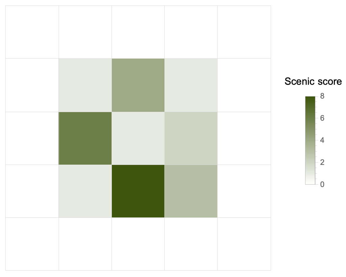
Part 2
Now things definitely get more complicated, because we have to find the best tree. How? According to a scenic score which is the product of four numbers, one for each side. Each number is the maximum distance along which we can admire the view without being blocked by taller trees.
We must have a function that, given a point (tree) and a list (its row/column “neighbors”), calculates the 4 distances. It increments a counter variable for each lower tree. As soon as it encounters an equal or taller tree, it stops and returns the counter, which will be the distance searched.
counter[value_][list_] :=
 Catch[
  list === {} && Throw[0];
  Block[{total = 0},
   Scan[Which[# < value, ++total, # > value || # == value,
      Throw[++total]] &, list];
   Throw[total]
   ]
  ]
Now we have two steps to get to the solution.
(1) For each point, we find once again the 4 lists of neighboring points (left/right, up/down):
Flatten[MapIndexed[pick[#2, forest] &, forest, {2}], 1]
pick is the middle portion of the VisibleQ function seen in Part 1. I have made it self-contained for simplicity. For instance, for the point (1, 1) of the example input, this function spits out something like: {3, {{}, {0, 3, 7, 3}, {}, {2, 6, 3, 3}}. The point (1, 1) corresponds to the height value 3 and:
(2) To apply the counter function3 we need a double Map: the first will scroll over lists like {p, {sx, dx, up, down}}. The second will apply counter` to each neighbor list, keeping the reference point fixed. It will come up with another list that will again be a matrix: each point-tree will be associated with the four distances, which, multiplied, will give the scenic score.
All that remains is to find the maximum of this list as a function of the product of the 4 distances. This is easy thanks to MaximalBy:
MaximalBy[
  Map[Map[counter[#[[1]]], #[[2]]] &,
   Flatten[MapIndexed[pick[#2, data] &, data, {2}], 1]],
  Apply[Times]
  ] // Flatten /* Apply[Times]
The last bit, Flatten /* Apply[Times], is just multiplying the resulting 4 values to obtain the scenic score.
😓 It is 23:38 and I have not yet had my evening herbal tea. I’m really starting to believe that I don’t think I will endure until Christmas with this frantic pace of finding the solution and writing the report. I’m going to try, though, as long as I keep up.
Bonus: maps

🎄👨💻 Day 7: No Space Left On Device
The dreaded day came, eventually. Without a little hint, I would not have been able to pull out the solution.
The problem was not that I didn’t have a clue on how to solve the puzzle, but that I was stuck with my first approach, refusing to change perspective. That is why the account of this seventh calendar day is perhaps the most important of all the previous ones. Because I found a difficulty that, at first, had completely blocked me. Then a change of point of view allowed me to find the correct solution.
Today’s problem, in short. The Elves’ apparatus has more than its messaging system malfunctioning. You attempt to execute a system update, but it does not go through since there is insufficient disk space available. You inspect the filesystem to examine what’s happening and record the terminal output generated.
The output is very similar to what you would get on a UNIX system. The cd and ls commands are used to change and list the contents of a directory. Each file is associated with its size in bytes (?).
Part 1
Since we have to try to free up space, the first thing to do is to calculate the size of each directory. One directory can contain others, and we have to take this into account to calculate the final size.
My initial idea was to build a data structure that was as similar as possible to the filesystem nested hierarchy. Each entity in this collection of elements had to contain, eventually, other entities (if it were a directory), or simply the name of the file and its size.
I therefore wrote this class:
class Dir:
    """A Dir class"""

    def __init__(self, name):
        self.name = name
        self.children = {}
        self.parent = None
        self.size = 0

    def add(self, child, value=None):
        """Add children to Dir"""
        self.children[child] = value

    def total(self):
        """Total size of this Dir"""
        if self.children:
            for child in self.children.values():
                self.size += child.total() if isinstance(child, Dir) else child
        return self.size

    def __repr__(self):
        return f"Dir({self.children}, parent: '{self.parent.name if self.parent else None}')"
The .total() method already does what one would expect: calculate the total of a directory, following recursively any nested directory. The real stumbling block I haven’t yet overcome was figuring out how to calculate the size of individual directories. Why? Because the puzzle clearly says that, for example, a baz.txt file in the /foo/bar/ directory will contribute to the size of both directories plus the root /. I swear I was unable to write the code that would allow me to do this simple operation.
I was taking too long, so I took a detour on YouTube and was inspired by a video by Jonathan Paulson, a competitive programmer who almost always manages to be in the top 100 people who solve both Advent of Code puzzles. I only had to listen to how he described the problem to figure out how to rewrite the solution. The idea was very simple: simply keep track of each path and its size in a trivial dictionary and without creating a nested object.
Here’s my second attempt with the parsing function:
from collections import defaultdict

def parse(puzzle_input):
    paths = []
    sizes = defaultdict(int)

    for line in puzzle_input.splitlines():
        words = line.strip().split()
        if words[1] == "cd":
            if words[2] == "..":
                paths.pop()
            else:
                paths.append(words[2])
        elif words[1] == "ls" or words[0] == "dir":
            continue
        else:
            size = int(words[0])
            for i in range(1, len(paths) + 1):
                sizes["/".join(paths[:i])] += size

	return sizes
For each line in the input, there are three action we can take:
The following bit of code it’s the interesting one. It’s where we add the size of the current file to all directories it belongs to. That is, to all of its parents up to /. We perform a loop over the parents paths, we build a nice UNIX-like path string, and then add the file size.
size = int(words[0])
for i in range(1, len(paths) + 1):
   sizes["/".join(paths[:i])] += size
Part 1 asks us to find all the directories that are at most 100 000 in size. That’s pretty easy with our sizes dictionary:
def part1(data):
    total = 0
    for size in data.values():
        if size <= 100_000:
            total += size
    return total
Part 2
The second part asks us to find the smallest directory that would allow running the upgrade. We know the total space available and the space required by the update. Thus:
avail = 70_000_000
needed = 30_000_000
max_used = avail - needed
free = data["/"] - max_used
The max_used is the maximum space we are allowed to use. The minimum space we need to free up is the total space we’re occupying, data['/'] – the space of the root directory – minus the allowed maximum. It means two operations: a filtering and then sorting.
def part2(data):
    avail = 70_000_000
    needed = 30_000_000
    max_used = avail - needed
    free = data["/"] - max_used

    candidates = list(filter(lambda s: s >= free, data.values()))

    return sorted(candidates)[0]
Day 7 is done, but I have to thank Jonathan Paulson because, without his hint, I doubt I would have been able to finish today. But that’s what happen when you’re trying to learn, right? You push yourself until it’s not longer easy and you’re stuck with a seemingly insurmountable difficulty. Then, with the help of someone more experienced or by studying the subject a little more, one is often able to overcome the stumbling block. And it is this experience that, as it accumulates, makes all the difference in the world in any learning process.
“Hey, Edoardo, do you have also a nice and elegant solution in the Wolfram Language?”
“Next time, my friend. Perhaps as a Christmas present. Now I’m pretty satisfied with what I got.”
🎄👨💻 Day 6: Tuning Trouble
The preparation phase is finally over, and the expedition in the jungle can begin. You and the Elves set off on foot, each with their backpack filled only with what you’ll need (hopefully). Suddenly, one of the Elves hands you a device. “It has fancy features,” he says, “but you need to set up its communication system right away.” He adds with a grin, ”I heard you know your way around signal-based systems - so this one should be easy for you!” They gave you an old, malfunctioning device that you need to fix. ‘Thanks a lot, friends!’
No sooner had he finished speaking, some sparks signals that the device is partially working! You realize it needs to lock onto their signal. To make it work as it should, you must create a subroutine that detects when four unique characters appear in sequence; this indicates the start of a packet in the communication data-stream.
Your task is clear: given an input buffer, find and report how many characters there are from its beginning to the end of that four-character marker.
Part 1
If we can scan the input and split it in overlapping subsequences of 4 chars, then we could compare them and find the first one that doesn’t contain duplicates characters. That one would be our marker string.
We need to have a utility function for that purpose. It should behave as if a four-characters wide windows scrolled over the string. The offset between one substring and the next is exactly one character. We also need to consider that we might end up with strings that are shorter than the target length if there are not enough characters left.
Here’s our partition() function:
def partition(l, n, d=None, upto=True):
    """
       Generate sublists of `l`
       with length up to `n` and offset `d`
    """
    offset = d or n
    return [
        lx for i in range(0, len(l), offset)
        if upto or len(lx := l[i : i + n]) == n
    ]
To obtain the solution, we need to transform each sublist into a set to remove any duplicates. Only the resulting sets whose length is still 4 characters are potential candidates for our marker string. We can filter out the others and take the first one. Then, find the index in the original string where our substring starts. Python has the str.find(substr) method for that precise purpose.
def part1(data):
    pdata = list(map(set, partition(data, n=4, d=1, upto=False)))
    marker = list(filter(lambda x: len(x) == 4, pdata))[0]
    return ("".join(data)).find("".join(marker)) + 4
Why are we summing 4 at the end? Because the puzzle asks for “the number of characters from the beginning of the buffer to the end of the first such four-character marker.”
Part 2
There’s a slight plot twist: we also need to decode the start of messages with another, appropriate marker. This time, the marker string is 14 characters long. Once again, our partition() function is versatile enough: we only need to change the offset argument to 14. The code is identical to Part 1’s.
My source of inspiration
As I was able to find the complete solution in a short time, I took some time to make some comparisons with another programming language. A particularly special language since it was the first one I learned: the Wolfram Language (now “WL” for short). For this kind of tasks, it really excels, I have to say. The idea of implementing the partition() function came from remembering that WL has an identical function with many, many more options.
The elegance of the solution written in WL is astonishing (but, as I said, I’m completely biased). I let the reader judge by themselves.
With[{sample = inputDay6},
 Flatten/*Last@
  StringPosition[sample,
   StringJoin@Select[
     Partition[Characters@sample, 4, 1],
     DuplicateFreeQ, 1]
   ]
 ]
🎄👨💻 Day 5: Supply Stacks
It’s starting to get serious today, at least as far as input parsing is concerned. The Elves are still in the process of unloading the materials needed for the expedition. On the cargo ship, the material is arranged in crates stacked in a certain order. It would be too easy (and unrealistic) if we could unload all the crates. The ones we need are scattered on the ship, piled in different groups.
The ship’s operator is quick to determining in what order to move the crates so as to retrieve those that the Elves need. They, however, forgetful as they are, do not remember which crates will be the ones they can unload first, that is, the ones that will be at the top of each stack at the end of the “sorting” procedure.
Part 1
The input is divided into two parts. The first, the different stacks with crates before the intervention of the operator. The second, the list of rearrangement operations. It is the first part that is problematic. The example input reads
    [D]
[N] [C]
[Z] [M] [P]
1   2   3
If the operator were to move 2 crates from the second to the third stack, for example, she will move one at a time. Which means that the order of the crates will be reversed: the first crate moved will end up as far back as possible in the stack to which it is moved.
In order to handle crate stacks as if they were lists, we need to find a way to convert a list like [[D], [N,C], [Z,M,P]] to [[Z,N], [M,C,D], [P]]. Unfortunately, this is not a simple transposition, but two operations are needed:
For the two steps to work, one more thing is necessary: you must keep the blanks. For example, the first line cannot be [ [D] ], but must be [ [blank, D, blank] ].
There is another problem to handle in parsing the input if we want the transpose operation to make sense: the array must be square, or at least rectangular.
The steps to parse the input are the following:
And now, the fun part. To process the stacks configuration and obtain our matrix, we need to:
I’m 99% sure that’s not the easiest or clearest way, but I had so much fun in trying to implement this matrix approach1. The problem resembles a lot the Hanoi Towers’ puzzle, and I bet there are hundreds of schemes or algorithms to solve it.
To obtain the answer to Part 1, we only need to process our stacks according to the list of moves. Remember: we must move the crates one by one. That’s easy enough now that we have our matrix of stacks:
def part1(data):
    stacks, moves = data
    for num, src, dest in moves:
        s, d, n = int(src) - 1, int(dest) - 1, int(num)
        for _ in range(n):
            stacks[d].append(stacks[s].pop())
    return "".join(map(lambda x: x[-1], stacks))
We also need to decrement all the indexes in each move because Python counts from zero. The return statement simply takes the topmost crate in each stack and then joins the characters to get the final answer 🎉.
Part 2
It has to be expected: it turns out that the “giant cargo crane” can move more than one crate at a time. Even better: as many as we want. The code change is minimal because the bulk of the work was reading and saving the crates stack in the right way.
The only thing that changes is that we don’t need the loop for _ in range(n) because we can move more than one crate at a time. We also cannot use pop() because it does not support a range, so we have to do it by hand: extract the elements we are interested in and then delete them.
def part2(data):
    stacks, moves = data
    for num, src, dest in moves:
        s, d, n = int(src) - 1, int(dest) - 1, int(num)
        stacks[d].extend(stacks[s][-n:])
        del stacks[s][-n:]
    return "".join(map(lambda x: x[-1], stacks))
It's 11:59 pm, and Day 5 is finally over. Unexpectedly tough.
🎄👨💻 Day 4: Camp Cleanup
Today the Elves start working for real: they need to clear the base camp to make enough space to unload the rest of the material for the upcoming expedition.
“Let’s divide the whole area to clear,” an Elf suggests.
“Good idea, let me take care of it,” another one replies.
So the enthusiastic Elf divides the sections and assigns them to the other Elves who will work in pairs. Each pair will work on two ranges of sections, for example 2,4-6,8: the first Elf will handle sections 2 to 4, the second from 6 to 8.
Unfortunately, the enthusiastic Elf made a bit of a mess. He didn’t realize he assigned overlapping ranges. So we have to find out how many sections are already contained in others, so that we can reassign them and avoid unnecessary work for the Elves.
Part 1
As on Day 3, the anatomy of the problem suggests using sets. We need to determine if a group of numbers is a subset of another or which numbers two groups have in common. Both of these operations are immediate with a set.
Perhaps the most interesting part of today’s puzzle is how to parse the input. We have:
2-4,6-8
2-3,4-5
5-7,7-9
...
and we want
[
 [[2,4], [6,8]],
 [[2,3], [4,5]],
 [[5,7], [7,9]],
 ...
]
We can do the first step of input parsing in one line (because it’s fun):
data = [
 list(map(lambda p: list(map(int, p.split("-"))), pair.split(",")))
 for pair in puzzle_input.splitlines()
]
The second step of the parsing phase is to build a “list of pairs of sets”, where each element of the pair includes all the IDs in the range. Here we need to consider one important detail: the ranges must include the last ID. Hence, we must increment by 1 the second element of each range, otherwise Python will ignore it. That’s a for loop and another map:
sets = []
for p1, p2 in data:
	# range must be inclusive
	p1[1] += 1
	p2[1] += 1
	p1, p2 = map(lambda x: set(range(*x)), (p1, p2))
	sets.append((p1, p2))
Once we did that, the solution to Part 1 is almost immediate: we only need to find if, in each pair, any set is a subset of the other, and count how many of these overlapping sets there are:
def part1(data):
    overlaps = 0
    for p1, p2 in data:
        if p1 <= p2 or p1 >= p2:
            overlaps += 1
    return overlaps
Part 2
The second part of the problem asks us to find (and count) those pairs of ID ranges that overlap for at least one ID. The total will necessarily be greater than the number found in Part 1. The way we read the input allows us to find the solution by changing only one line from Part 1:
def part2(data):
    overlaps = 0
    for p1, p2 in data:
        if p1 & p2:
            overlaps += 1
    return overlaps
🎄👨💻 Day 3: Rucksack Reorganization
It’s a classic problem of those who are not used to hiking: preparing a backpack and carrying only what is necessary, no extra unneeded stuff.
The Elves made a big mess with the backpacks. Each backpack has two equal compartments, and there is a finite list of items that they can bring with them. Our input is the list of contents of the backpacks. Each line is a string in which each character represents an item class. Some people put more stuff and some put less, but the two compartments contain the same number of items. The problem is that the person who made the backpacks put some items of the same type in both compartments. That’s unnecessary weight.
Part 1
Not all elements have equal priority, and we have to calculate the total priority of those elements that are present in both compartments. We know that there is only one class of items.
The priorities are calculated simply according to alphabetical order. Elements labeled a-z have priorities 1-26, while those A-Z will have 27-52. We can construct a dictionary on the fly that contains each element with its priority:
# a-z and A-Z letters
from string import ascii_lowercase, ascii_uppercase

prios = {letter: prio for prio, letter in \
         enumerate(ascii_lowercase + ascii_uppercase, start=1)}
The gist of the problem is an intersection operation between the two compartments of each backpack. And again, everything is already built-in into Python thanks to sets1. Thus:
Part one’s solution is the sum of all priorities:
def part1(data):
    """Solve part 1"""
    total = 0
    for line in data:
        mid = len(line) / 2
        first, second = set(line[:mid]), set(line[mid:])
        total += prio[(first & second).pop()]
    return total
Using .pop() seems to be naive as the resulting set will have only one element, but a standard set doesn’t support indexing2.
Part 2
We know that the Elves will take part in the expedition in groups of three. Each group splits the load into the three backpacks, but there is one item that each Elf must always have: their badge. Each trio will have a badge indicated with a different letter, but we do not know which letter each group’s badge corresponds to.
Since each Elf has only one badge, we need to find which item’s class is present in all their backpacks. Instead of the compartments of a single backpack, we must consider the entire contents of the three backpacks in the group:
def part2(data):
    """Solve part 2"""
    total = 0
    i = 0
    for line in data[::3]: # we jump by 3 lines
        group = set(line) & set(data[i+1]) & set(data[i+2])
        total += prio[group.pop()] # same thing as in Part 1
        i += 3 # don't forget to increase the counter!
    return total
I suspect that the for loop with the manual counter isn’t the best way to implement that logic, but I didn’t come up with a better solution (for the moment).
🎄👨💻 Day 2: Rock Paper Scissors
Second day, second warm-up.
The Elves are setting up base camp before venturing into the jungle. To decide who will get the best-positioned tent – that is, the one closest to the food supply meticulously calculated yesterday – the Elves are holding a Rock-Paper-Scissors tournament. The rules are the standard ones, but the scoring will be done as follows:
The input is the secret key provided to us by a friendly Elf so that we can easily win the tournament. There’s not much structure and it’s quite easy to parse, only a bunch of rows with two letters.
Part 1
The problem is on the interpretation of the input: we do not know what the second column indicates, where X, Y, and Z stand for rock, paper, and scissors.
We make an hypothesis: if the second column represents our choice during a single match, then we need only add the value associated with the character (A=1, B=2, C=3) in the second column to that of the outcome of the game.
def part1(data):
    """Solve part 1"""
    POINTS = {"X": 1, "Y": 2, "Z": 3}

    total_points = 0

    for line in data:
        opp, me = line.split()
        total_points += POINTS[me]
        if opp == "A":
            if me == "X":
                total_points += 3
            elif me == "Y":
                total_points += 6
        elif opp == "B":
            if me == "Y":
                total_points += 3
            elif me == "Z":
                total_points += 6
        else:
            if me == "Z":
                total_points += 3
            elif me == "X":
                total_points += 6

    return total_points
Part 2
There’s a second possibility, which turns out to be the correct one: the second column means the outcome that the game needs to have. In fact, it would be very suspicious if we won every game; someone would suspect that we are cheating (as we are).
In this case, we already know the score of the final outcome – that’s the score associated to X (0, lose), Y (3, draw), and Z (6, win). We have to find which choice between rock-paper-scissors will produce that outcome. The first column always represents our opponent’s choice.
We only need a couple more if...else, but the solution is fairly easy:
def part2(data):
    """
    Solve part 2

    X = lose
    Y = draw
    Z = win
    """
    ENDS = {"X": 0, "Y": 3, "Z": 6}

    total_points = 0

    for line in data:
        opp, end = line.split()
        total_points += ENDS[end]
        # lose
        if end == "X":
            if opp == "A": # rock
                total_points += 3
            elif opp == "B": # paper
                total_points += 1
            else:
                total_points += 2
        # draw
        elif end == "Y":
            if opp == "A": # rock
                total_points += 1
            elif opp == "B": # paper
                total_points += 2
            else:
                total_points += 3
        # win
        else:
            if opp == "A": # rock
                total_points += 2
            elif opp == "B": # paper
                total_points += 3
            else:
                total_points += 1

	return total_points
A very elegant solution (not mine)
One could say very Pythonic. It takes full advantage of the versatility of dictionaries1 and the sum operation between two strings which means to concatenate.
First, we create a dictionary that stores the values of the single choices (A=X=1, B=Y=2, C=Z=3) and the 9 possible outcomes (AX, AY, AZ, etc…).
points = dict(X=1, Y=2, Z=3,
             AX=3, AY=6, AZ=0,
             BX=0, BY=3, BZ=6,
             CX=6, CY=0, CZ=3)
The first part is practically solved in one line, without even an if...else block:
total_points = sum(points[me] + points[me + opp]
				   for opp, me in [line.split()
				   for line in open('input.txt').readlines()])
Wow 🤯.
🎄👨💻 Day 1: Calorie Counting
The first day - maybe the first week - is just warming up. It serves to get us back into the mood, a Christmas-flavored atmosphere that is anything but passive: it is not the awaiting of something or someone that is supposed to come, but a road that will get steeper day by day to make us sweat out the 25 stars before Christmas.
In this year’s adventure, the Elves are on an expedition to a mysterious island to retrieve Santa’s reindeers favorite food, food that contains the indispensable “magic energy”. There will be a jungle to traverse, so let’s get ready for some obstacle running or mazes among the trees.
Part 1
The Elves sort the food they brought with them and want to make sure they have enough. We need to count how much food each Elf brings. The puzzle input divides each Elf’s rations into blocks separated by blank lines. So here’s how to read the input: divide it at the blank lines and convert everything to integers.
lines = [
    list(map(int, line.strip().split("\n")))
    for line in re.split(r"^$", puzzle_input, flags=re.M)
]
We’ll end up with a list of lists. To find the solution, it suffices to sum up each sub-list, and then find the largest sum of all.
A quick explanatory note: we used the re.split() method (from the re standard library package) to be able to split the input at every empty line, represented by the regex ^$. The flag re.M (which is a shortcut to re.MULTILINE) is important to match each empty line. Otherwise ^$ would match the start/end of the whole string only.
sums = sorted([sum(l) for l in lines], reverse=True)
print(sums[0]) # the largest sum
Part 2
The Elves want to know the three in the group who have the most food, to make sure that no one will run out of food during the expedition. The solution is straightforward: all we have to do is pull out the first three items from the list of sums obtained in Part 1 (i.e., the top three), and then add up these three numbers. It’s as easy as
print(sum(sums[:3]))