🎄👨💻 Day 8: Treetop Tree House
Eric keeps raising the bar with a problem that made me disown Python because otherwise I would have took much longer. I started sketching the solution with the Wolfram Language and wanted to finish the whole puzzle. I will try to recount the highlights of the code that, by the way, earned me today’s stars.
Part 1
The Elves’ project is to build a cozy treetop house. It is not clear how much time they have for this expedition, but so be it. The vast forest in which they find themselves covers a fairly regular area, and the Elves are able to reconstruct a two-dimensional map of it in which each tree is represented by its height1, from 0, the lowest height they have been able to measure, to 9.
The Elves first want to determine where it would be ideal to build the tree house. They need to find the most hidden location possible. They ask us to determine how many trees are visible to an observer outside the forest. A tree is visible if all other trees between it and the forest boundaries are shorter than it. It’s clear that all trees at the edges of the forest will always be visible, so we can already discard them as possible candidates (but we will come back to this in Part 2).
Reading the input is rather simple today: it’s a list of strings with integer digits from 0 to 9. We need to read it in as a matrix of integers:
Map[FromDigits, Characters /@ StringSplit["input.txt", "\n"], {2}]
Given a grid point, we must consider the points to the right, left, top, and bottom, and determine which trees are lowest. A tree will be visible if at least one of these “forest segments” contains only lower trees in height.
For each point (i, j), the row and column containing it will be row = forest[i][:] and col = forest[:][j]2.
From row and col we need to extract two sets of points: those to the right/left and above/below the point under consideration, excluding the point itself. The Wolfram Language has a dedicated function: TakeDrop[list, n] returns two lists, one containing the first n elements, and the second those remaining.
Here is the first piece of the function for the first part ((x, y) are the coordinates of the point):
With[{row = matrix[[x, ;;]], col = matrix[[;; , y]]},
 {sx, dx} = TakeDrop[row, y];
 {up, do} = TakeDrop[col, x];
]
The procedure for looking for visible trees could be put into words like this: look along the row, right then left, and check for all lower trees. Repeat along the column, up then down. The important logic is as follows: in the right/left (or top/bottom) direction, all trees must be lower than the one we’re considering. But only one part of a row/column must meet the criterion for the tree to be visible.
Here is the complete function that, given a point p, its coordinates, and the matrix-forest, tells us (True/False) whether the tree is visible:
VisibleQ[p_, {x_, y_}, matrix_] :=
 Block[{sx, dx, up, do},
  With[{row = matrix[[x, ;;]], col = matrix[[;; , y]]},
   {sx, dx} = TakeDrop[row, y];
   {up, do} = TakeDrop[col, x];
   AllTrue[Most@sx, p > # &] ||
    AllTrue[dx, p > # &] ||
    AllTrue[Most@up, p > # &] ||
    AllTrue[do, p > # &]
   ]
  ]
We just need to apply it to every point in the matrix-forest. Here we have to pull another gem out of Wolfram’s hat: MapIndexed. It does the same thing as Python map(), but it also passes the indices of the current list item to the function to be mapped. A trivial example:
MapIndexed[f, {a, b, c, d}]
(* {f[a, {1}], f[b, {2}], f[c, {3}], f[d, {4}]} *)
And it works with objects of any size! We just need to specify at what level we want to apply the function.
Count[
 MapIndexed[VisibleQ[#1, #2, forest] &, forest, {2}],
 True, {2}
 ]
Part 2
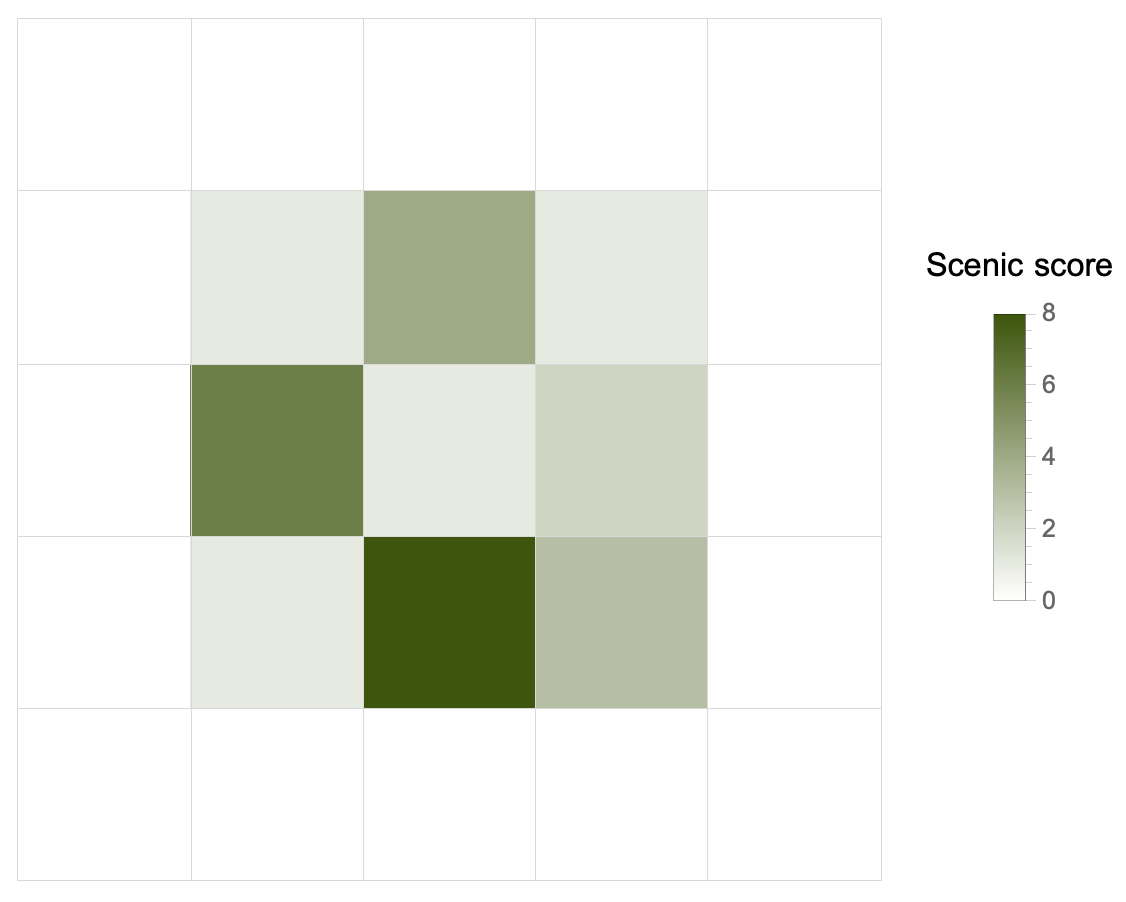
Now things definitely get more complicated, because we have to find the best tree. How? According to a scenic score which is the product of four numbers, one for each side. Each number is the maximum distance along which we can admire the view without being blocked by taller trees.
We must have a function that, given a point (tree) and a list (its row/column “neighbors”), calculates the 4 distances. It increments a counter variable for each lower tree. As soon as it encounters an equal or taller tree, it stops and returns the counter, which will be the distance searched.
counter[value_][list_] :=
 Catch[
  list === {} && Throw[0];
  Block[{total = 0},
   Scan[Which[# < value, ++total, # > value || # == value,
      Throw[++total]] &, list];
   Throw[total]
   ]
  ]
Now we have two steps to get to the solution.
(1) For each point, we find once again the 4 lists of neighboring points (left/right, up/down):
Flatten[MapIndexed[pick[#2, forest] &, forest, {2}], 1]
pick is the middle portion of the VisibleQ function seen in Part 1. I have made it self-contained for simplicity. For instance, for the point (1, 1) of the example input, this function spits out something like: {3, {{}, {0, 3, 7, 3}, {}, {2, 6, 3, 3}}. The point (1, 1) corresponds to the height value 3 and:
- on the left, it has no neighbors (it’s on the left border);
- on the right, it has
{0, 3, 7, 3}, in that exact order; - it has no neighbors above (so it’s in the upper right corner);
- it has
{2, 6, 3, 3}below.
(2) To apply the counter function3 we need a double Map: the first will scroll over lists like {p, {sx, dx, up, down}}. The second will apply counter` to each neighbor list, keeping the reference point fixed. It will come up with another list that will again be a matrix: each point-tree will be associated with the four distances, which, multiplied, will give the scenic score.
All that remains is to find the maximum of this list as a function of the product of the 4 distances. This is easy thanks to MaximalBy:
MaximalBy[
  Map[Map[counter[#[[1]]], #[[2]]] &,
   Flatten[MapIndexed[pick[#2, data] &, data, {2}], 1]],
  Apply[Times]
  ] // Flatten /* Apply[Times]
The last bit, Flatten /* Apply[Times], is just multiplying the resulting 4 values to obtain the scenic score.
😓 It is 23:38 and I have not yet had my evening herbal tea. I’m really starting to believe that I don’t think I will endure until Christmas with this frantic pace of finding the solution and writing the report. I’m going to try, though, as long as I keep up.
Bonus: maps
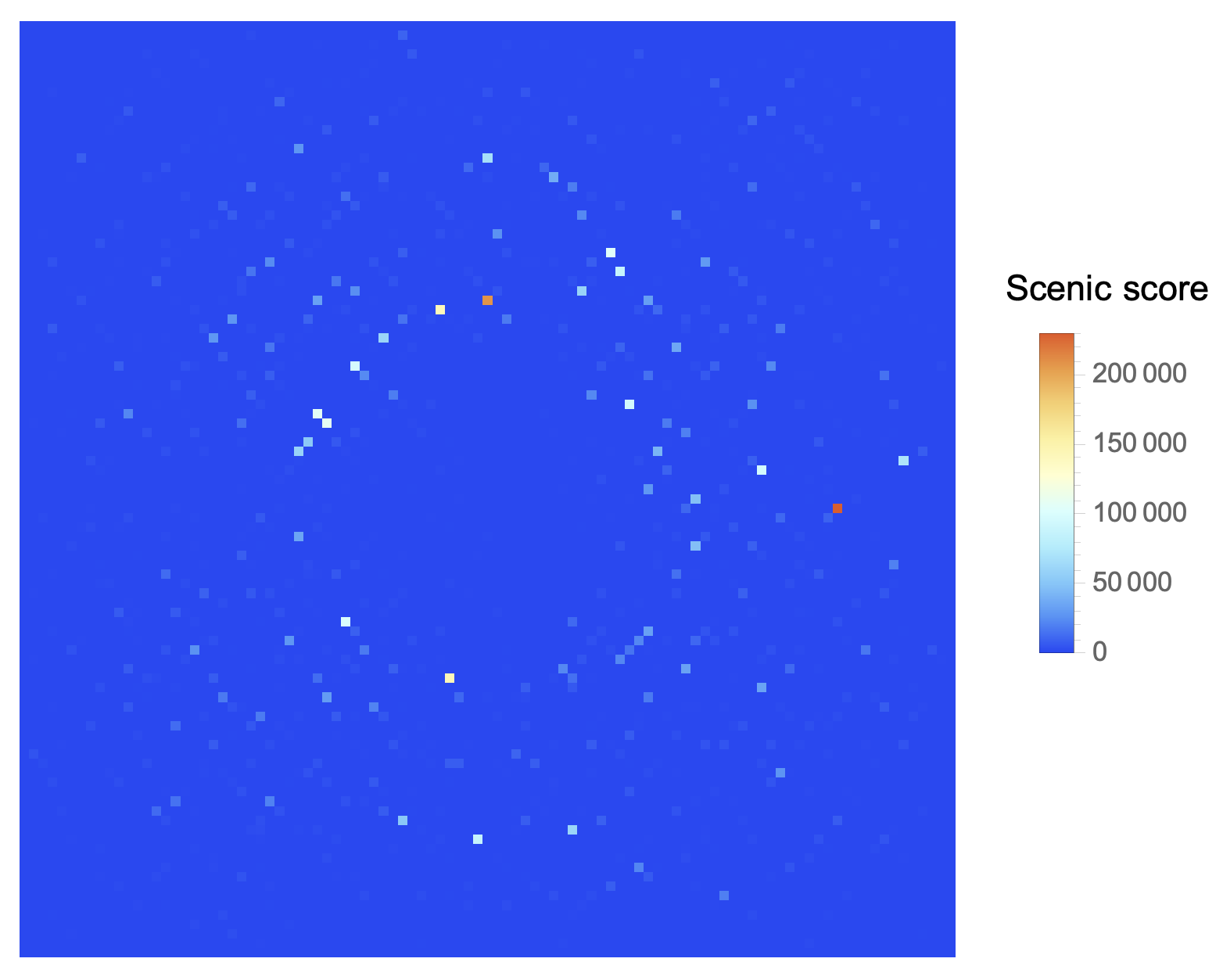
-
A perfect representation of a field in physics. Inevitable note because the writer is proud of his scientific background, although he likes a lot computer science stuff. ↩︎
-
This is not the right way to slice a 2D list in Python; it’s pseudo-code to give an idea. ↩︎
-
Or at least in the way I wrote it. I thought of simplifying it to allow a clearer application, but I didn’t have time today. I’m sure I’ll go through these notes once again in the future, also because I want to write a Python solution as well. ↩︎