Santiago #4: nel cuore della Navarra
Il quarto giorno si arriva a Pamplona, capoluogo della Navarra e la città più grande che si incontra sul Cammino Francese. Tappa di poco più di 20 km – perlopiù in piano – che si è rilevata più tosta del previsto. Vista la stanchezza, il diario vocale torna domani, promesso.


Santiago #3: quando ci sentiamo davvero a casa?
Santiago #2: quanto mi costerà?
Santiago #1: Le motivazioni di un viaggio
Santiago #0: la partenza è già un viaggio

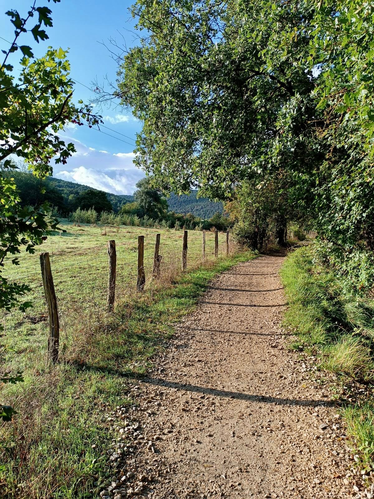
In mezzo alla campagna francese, partiti da Bordeaux verso Bayonne – o Baiona in basco e spagnolo – l’ultima fermata intermedia prima del paese pirenaico di Saint-Jean-Pied-de-Port (o SJP d’ora in poi), il vero punto di partenza di questo Cammino Francese.
Dopo la tempesta ancora estiva che ci ha accolti ieri all’atterraggio a Bordeaux, la giornata oggi è pulita e fresca, la notte è stata tiepida e invoglia a passare la prossima in tenda.
Abbiamo già fatta una conta degli zaini incrociati fino a stamattina e ci siamo chiesti quanti ne rincontreremo alla vera partenza. Previsione? Un buon cinquanta percento, e ne avremo visti almeno una trentina. Ciò è un buon segno perché la condivisione con altri esseri umani è per entrambi uno dei motivi che ci ha portato su questo sentiero frequentatissimo.
L’umore è alto – e contrasta un po’ con l’atmosfera lavorativa che avvolge la carrozza di questo TGV – l’energie pure, pronte a servirci in questo inizio che sarà una bella tappa alpina, come piace a noi.
Appuntamento a più tardi per la prima puntata del “diario vocale” di questo Cammino. Parleremo di motivazioni personali e di quanto contano (e costano) 🥾
I’m seriously thinking of camping here next weekend 🏕️ I know this place since ages but I can’t deny a pinch of fear of I don’t know what

La sorpresa di un cambio di prospettiva

Dopo la prima giornata, una tappa abbastanza impegnativa come inizio, la scenografia delle Dolomiti di Brenta ci ha regalato un piccolo insegnamento sulla sorpresa di un banale cambio di prospettiva.
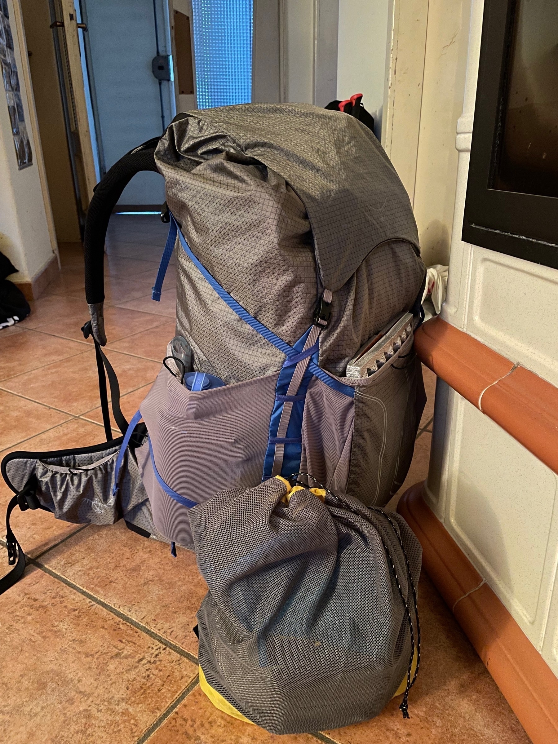
The real thing
Before removing the yellow bag it was 9.1 kg. I think I did even better with the help of an expert.
Ci nutriamo davvero di energia?
Farò un excursus che sembra c’entrare molto poco con un trekking in montagna, ma credo invece che sia perfettamente in tema. Ci ho pensato proprio ieri pomeriggio quando mi sono messo a preparare tutti i pasti che dovranno sostentarmi nei prossimi giorni. Contando tutte le chilocalorie che stavo impacchettando, mi sono chiesto1: ma mi serve davvero l’energia contenuta in queste barrette o tortilla al burro d’arachidi? Serve essere un po’ più pignoli se vogliamo trarne un ragionamento abbastanza preciso. Seguitemi un attimo (se v’interessa).

Alla domanda “qual è la caratteristica essenziale di un essere vivente” potremmo rispondere brevemente con una parola: metabolismo. L’origine è dal greco, e significa “cambiare”. O meglio: scambiare. Scambio di che cosa? I candidati più ovvi sono due: materia o energia2.
Sulla materia, è facile capire perché non può essere ciò che caratterizza il nostro metabolismo. Ogni atomo di idrogeno, ossigeno, o carbonio contenuto in una barretta energetica o un maccherone al formaggio è assolutamente identico a un qualunque atomo di idrogeno, ossigeno, o carbonio che espelliamo nelle nostre maniere abituali (sudore, respirazione, deiezioni). Come potrebbe lo scambio di entità perfettamente identiche permetterci di vivere, ossia di distinguerci da un pezzo di materia inanimata?
Se non è una, è l’altra, ma non è così semplice. L’energia è un concetto strano e complicato. Non abbiamo una buona definizione di energia3 che non sia un modo preciso di calcolarla. E sappiamo calcolare benissimo anche la più piccola quantità di energia che si libera o viene assorbita in moltissimi processi della nostra epoca industrializzata. Sappiamo anche un’altra cosa, una delle leggi più fondamentali che esistano, un decreto inviolabile della natura: l’energia si conserva, non possiamo distruggerla.
Pensare che il nostro metabolismo sia lo scambio di energia è solo in parte corretto. Se non possiamo distruggere nessuna quantità di energia, e ovviamente ogni singola unità di energia – per esempio, una chilocaloria della nostra barretta – è equivalente a qualunque altra, dove sta il vantaggio? Che cos’è che scambiamo davvero? La risposta qui è davvero in un dettaglio minuscolo, ma non possiamo andare avanti se non citiamo il secondo decreto più inviolabile dell’universo. Possiamo riassumerlo così: l’energia si conserva, ma non è tutta uguale. Ci sono forme di energia che sono più utili di altre. E il secondo decreto stabilisce che, sempre e comunque, nel nostro metabolismo o in qualunque altra trasformazione, sarà inevitabile produrre un po’ di energia completamente inutile.
Dovremo quindi essere più precisi: il nostro metabolismo ci permette di prelevare energia utile da una gustosa (si fa per dire) barretta al burro d’arachidi, consente alle nostre fibre muscolari di contrarsi innumerevoli volte e a impulsi elettrici di attraversare le nostre sinapsi, e poi scambiare una certa quantità di energia inutile con l’ambiente che ci circonda. Ci sarebbe addirittura un legame tra la nostra temperatura corporea e la particolare efficienza nel liberarci di questa energia inutilizzabile.
So che parlare di energia utile potrebbe non aiutare molti a capire. “Non bastava semplicemente chiamarla energia e lasciar perdere questo discorso?” Certo, a patto di voler raccontare solo una parte della storia. Ma per poterci liberare del termine “energia utile” dovremmo andare ancora un po’ più a fondo e cominciare a parlare di entropia – e io devo ancora finire di preparare lo zaino per domani 😅. Voglio però concludere con le parole4 di uno dei più importanti fisici del ‘900, Erwin Schrödinger, che non aveva certo problemi a tirare in ballo l’entropia per spiegare di che cosa ci nutriamo davvero.
Che cosa c’è di così prezioso nel nostro cibo che ci impedisce di morire? A ciò si risponde facilmente. Ogni processo, evento, cambiamento – chiamatelo come volete; in altre parole, qualunque cosa accada in Natura implica un aumento dell’entropia nella parte di universo in cui ciò accade. Un organismo vivente produce costantemente entropia positiva, e perciò si avvicina al pericoloso stato di massima entropia, cioè la morte. L’unica maniera in cui può evitarlo, cioè rimanere in vita, è assorbire entropia negativa dall’ambiente circostante.
Ecco quindi una risposta alla domanda iniziale: non di energia vive l’uomo, ma di entropia negativa.
-
Non sono certo il primo a farsi questa domanda, anzi. Buona parte dei fisici di fine ’800 e del secolo scorso hanno ragionato sulle implicazioni di una domanda analoga. ↩︎
-
Immagino che a molti sia risuonato in testa il nome di Einstein per via della sua formula più famosa, ma in questo caso potete dimenticarvela: non ci serve a nulla. ↩︎
-
Si potrebbe citare James Clerk Maxwell, che nel suo Theory of Heat (1872) scriveva che l’energia è “la capacità di compiere lavoro, [ossia] l’atto di produrre un cambiamento nella configurazione di un sistema contrastando una forza che si oppone a tale cambiamento”. È utile? Non molto, secondo me. ↩︎
-
Il passo è tratto dal libro What is life?, capitolo 6, pag. 72 della versione inglese (Cambridge University Press, 1967). La traduzione è mia. ↩︎
The theory
We’re only two days away from my (first) Translagorai1. I’ve put off writing this page for weeks, if not months. I told myself several times that I had an idea for how I might resume blogging about the next hiking trip I was preparing. And, even though I am not superstitious, I am not going to discuss one of the primary reasons I am currently here preparing for this journey. This Translagorai is, in many ways, the test for which I have been training physically and emotionally since February. It is one of the projects I am most excited about this year.
Last year, I also walked across the Trentino mountains, but if it is true (and often it isn’t) that we learn from our mistakes, I wanted to do better this year. And one thing I’ve learnt is that backpack weight is a crucial number. It might decide the fate of even the most modest trekking adventure. It can make the experience excruciating; you might come home uninjured, but if that number was higher than necessary – often because of a mix of absolutely unnecessary material – you might come home with a hamstring problem you will take months to recover from.
As a spreadsheets nerd, I did things correctly from the start. Every piece of gear, clothes, or other item that aspired to fit in my pack would be weighed (a few times, so I could get a reliable average 🤓). Also, when I chose to embark on the hike, I realized I’d need to improve a lot of my gear, specifically my backpacking gear (sleep system and backpack above all). So I separated everything into eight categories and methodically weighed everything – or estimated the weight based on the information I had. Here’s the result:
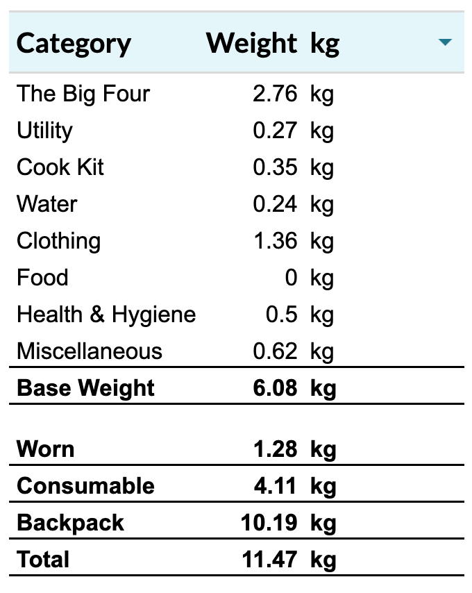
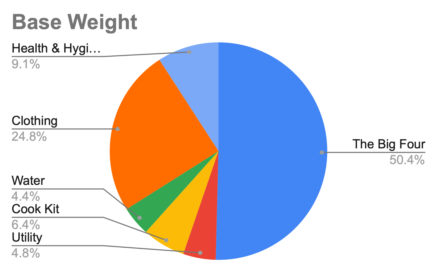

Although I may have overlooked something (hopefully minor), I’m pretty proud to have reached a base weight of roughly 6 kg. I was probably around 9 or 10 kg last year – and we didn’t even have a tent! So, why the theory? Because, in some ways, that weight doesn’t exist until it’s on my shoulders. That’s what I’ve been wondering since I entered the figures in that spreadsheet: will I be able to carry that weight for five days in a row?
-
For whoever didn’t know about the Translagorai trail, here’s a map with several hikes in the area, including a description of the thru-hike. ↩︎
🎄👨💻 Day 14: Regolith Reservoir
I’m now pretty confident: I have the most problems with the implementation of an algorithm that has to do with some kind of geometry. After Day 12 and finding the path on a map using graphs, Day 14 gave me just as many troubles. I also dedicated less time on it than usual and ended up not even completing the first part1. I will give a brief account of what my approach was, and keep these notes for when I return to write a complete solution.
We ended up in a cave opening behind a huge waterfall, the point to which the signal we deciphered yesterday led us. We immediately notice that something is wrong: it is raining sand in the cave. This is not comforting, so we attempt to make a quick simulation of where and how much sand may accumulate.
We have a scan of a vertical section of the cavern; or rather, of the part of the cave above us. It is full of tunnels through which the sand is threaded. The input is just the geometry in two dimensions of these burrows. We have a series of (x, y) points that show us the rock barriers. The + indicates the point where the sand enters and has coordinates (500, 0).
......+...
..........
..........
..........
....#...##
....#...#.
..###...#.
........#.
........#.
#########.
Sand, falling in small units occupying exactly one slot of the grid, accumulates according to three rules:
- It falls straight down until it meets the first obstacle, whether sand or rock.
- If it cannot occupy the lowest slot directly along its falling path, it slides left and then down (thus
-x → +y). - If the slot on the left is not available either, it slides to the right (
+x → +y).
In the example above, after 5 units of sand, we are at this point:
......+...
..........
..........
..........
....#...##
....#...#.
..###...#.
......4.#.
....5213#.
#########.
I have gone so far as to write a function that returns rock line paths. The puzzle input gives us the extremes of each line of rocks:
def rock_line(x1, y1, x2, y2):
    """Create a line of rock points between (x1, y1) and (x2, y2)"""
    rline = []
    x1, x2, y1, y2 = map(int, (x1, x2, y1, y2))
    delta = max(abs(x1 - x2), abs(y1 - y2))
    for i in range(delta):
        rline.append([x1 + (x2 - x1) * i / delta, y1 + (y2 - y1) * i / delta])
    return rline
The idea now would be to build a complete map of the cave that is basically a sparse matrix: everywhere zero except the locations where we know there is rock. Then, we will need to have a function – recursive once again – that will try to get other units of sand in following the rules above. When it finds the correct position, it will change an array value from 0 to 1.
The function will then iterate over the previous result until the map itself no longer changes. At that point, we know we can no longer add sand. Any extra amount will slide into the void, that is, to the sides of the pattern shown above. The symbol ~ below indicates a unit of sand that will fall indefinitely:
.......+...
.......~...
......~o...
.....~ooo..
....~#ooo##
...~o#ooo#.
...~###ooo#.
..~o.oooo#.
.~o.ooooo#.
~#########.
~..........
~..........
~..........
Post-scriptum
Perhaps I had little motivation today, who knows for what reason. The frenzy of Advent of Code is both a motivating drive and a risk of getting overwhelmed by wanting to get to the end at all costs. The goal is to practice how to approach a problem and, more importantly, how to translate a solution into an algorithm.
I realize that, without a formal education in computer science, I am missing several fundamental concepts that are essential tools for solving problems of this kind. For any aspiring programmer, it’s mostly a matter of practice, practice, and more practice – literally. We must get our heads used to seeing the logic of the solution before we put our hands on the keyboard.
How to have more practice – or rather, more sensible practice that does not make us prey to the anxiety of having to figure it all out by Christmas? Eric Wastl suggested a solution in a tweet about a year ago: there are 25 puzzles in the calendar. A year has 52 weeks. Why not read a puzzle every two weeks, so as to give yourself time (at least for the more complex ones) to tackle a complicated problem? In two weeks there is also time to study a bit. I might think of doing something like this from next year, although the Christmas spirit will have already waned.
-
I found the numeric answers to the puzzle, but by disassembling and reassembling someone else’s solution written in the Wolfram Language. If I don’t get to the solution by my own conceptual and implementation efforts, then it counts for very little. The two stars have no gusto. ↩︎
🎄👨💻 Day 13: Distress Signal
Hello, recursion! At last, we meet. On day 13, having abandoned harassing monkeys and algorithms on graphs to find the best paths1, we are grappling with deciphering a help message.
Part 1
Our multi-function device still does not seem to be working properly, despite having a screen that allows it to display as many as 8 characters. We soon discover that we receive the signal packets in a random order. Our (first) task is to find which pairs of packets are in the correct order. But order according to what criteria? Here are the first lines of the example input:
[1,1,3,1,1]
[1,1,5,1,1]

[[1],[2,3,4]]
[[1],4]
Packets are represented by lists that can contain either integers or other lists. We have to compare pairs of elements for each packet, and there are three rules for establishing an order:
- If they are integers, the order is the usual one: smaller numbers will come first. In the first case of the example, 1 vs. 1 is not decisive, but 3 vs. 5 is obvious.
- If both elements are lists, we compare their elements one by one. If the first list contains an integer greater than its corresponding one in the second list, then the order of the packets is wrong. If the first list contains fewer elements than the second, the order is correct (and will be incorrect vice versa). If the order cannot be determined, we must continue with the next part of the input.
- If only one of the two elements is an integer and the other is a list, we must convert the integer to a list (like
1 → [1]) and retry the comparison.
It is clear that the gist of the solution to this problem will be the function that performs the comparison. Such a function will inevitably be a recursive function.
Reading the input presents no particular difficulty, but we must find an agile way to read strings that look like lists as objects of type list. To do this, we have the built-in function eval() whose “argument is parsed and evaluated as a Python expression”2.
The result will be an array (list of lists), each row a pair of packets, whatever composition we have. Now for the interesting part. We need to loop over this array and compare the individual pairs. We need to remember the three rules above to understand how the function should behave, which is as follows:
def compare(p1, p2):
    """Compare two packets"""
    # (1) check if both args are integers
    if isinstance(p1, int):
        if isinstance(p2, int):
            # < 0 means correct ordering
            # 0 means undefined
            # > 0 wrong ordering
            return p1 - p2
        # (2a) 'p2' must be a list, but 'p1' is not
        p1 = [p1]

    # (2b) 'p1' must be a list
	#      'p2' must be as well if it's not already
    if isinstance(p2, int):
        p2 = [p2]

    # (3) recursively compare two lists
    for x, y in zip(p1, p2):
        if (r := compare(x, y)):
            return r

    # (4) compare lengths
    return len(p1) - len(p2)
(1) The first part compares the two arguments if they are both integers. In that case, it returns their difference (we will see in Part 2 why it will simplify our lives).
(2a) If the second argument p2 was not an integer, then we need to convert p1 to a list.
(2b) If p1 were not an integer, then we need p2 to be a list. We convert p2, in case it is not already a list.
(3) With two lists, we need to start going down a level until we have two integers in hand. That is the only direct comparison we can always make. We do a for loop that again takes pairs of elements from p1 and p2. If, at some point, it returns a value different from 0, i.e. True (in Python False is 0), then that value is the result of the comparison. Otherwise, it means the elements don’t have an intrinsic ordering.
(4) Finally, lists of different lengths (even nested list with empty elements like [[[]]] vs [[]]) determine an order (shorter vs longer is correct). Again, we calculate the difference in lengths: negative number means correct order, positive wrong order.
The first part ends with a loop – which can certainly be rewritten in a more elegant and compact way:
def part1(data):
    right_order = []

    for i, pair in enumerate(data, start=1):
        if compare(*pair) < 0:
            right_order.append(i)

    return sum(right_order)
Part 2
Now we must sort all the packets, including two extra ones: [[2]] and [[6]]. We must then find the indexes these two packages have in the ordered set of packages and multiply them together.
First, we need a simple list of packets, not a list of pairs (i.e., the matrix we have been working with so far). Again, this can be written much better3:
unroll = []
# add the extra packets
unroll.extend([[[2]], [[6]]])

for x, y in data:
	unroll.extend([x, y])
At this point, all we need to do is sort this new list. Python already has built-in the sorted() function (or the in-place .sort() method). But we discover one thing that doesn’t work: the key parameter of sorted accepts a single argument function, while our compare() takes two.
The key function, in essence, converts the elements of the array to a numeric value that is then used as the “ordinal criteria”. We would have to write a conversion between key and compare(), except that… it already exists! It is part of the functools module and is called cmp_to_key(): it takes a two-argument function and returns4 another function that can be passed as the key. The hidden gems of Python’s standard library.
def part2(data):
    unroll = []
    # add the extra packets
    unroll.extend([[[2]], [[6]]])

    for x, y in data:
        unroll.extend([x, y])

    unroll.sort(key=cmp_to_key(compare))

    return (1 + unroll.index([[2]])) * (1 + unroll.index([[6]]))
One crucial point of the cmp function to be converted into a key function: it must return a negative value for less-than, zero for equal, and a positive value for greater-than. That’s the reason to write compare() as I did, and not as a function returning True/False.
-
Alas, graphs are a subject about which I know almost nothing. I left aside the problem of Day 12 as a “holidays assignment.” I will study more and come back with the solution in due time. ↩︎
-
From the official documentation of Python. ↩︎
-
Or use
itertools.chain, which I discovered today. So much can be learned! ↩︎ -
A small bonus, useful as a future reference. Here is the CPython implementation of the
itertools.cmp_to_keyfunction. Another tidbit to keep in mind. ↩︎
🎄👨💻 Day 11: Monkey in the Middle
It wasn’t enough to have risked our lives by falling off a rope bridge into the river flowing in the gorge below. Now we met a group of nasty monkeys who are taunting us by throwing the stuff from our backpack. As we try to figure out how to intervene, we are quite apprehensive about our belongings and assign a certain worry level to each item. The monkeys handle each object a bit and then throw it at each other based on how they see us worrying. Each monkey may show a different interest in our objects, and its actions may increase our worry level a little or a lot.
Part 1
The notes we took on the annoying primate pastime take this form:
Monkey 0:
  Starting items: 79, 98
  Operation: new = old * 19
  Test: divisible by 23
    If true: throw to monkey 2
    If false: throw to monkey 3
Each monkey examines a single item on her list, plays with it, and this will change the worry level according to the indicated operation. Then, according to the result, the monkey will choose whom to pass it to. Each turn of the game ends when all monkeys have gone through all the items they have. It’s thus possible that one monkey will end up with no items, or that another monkey who had none at the beginning of the turn will end up with some to play with.
At first, we tell ourselves that this is not such a big deal. As long as the monkeys don’t damage our stuff, we manage to keep our worry level under control. Before each monkey passes an object to another, our worry level is divided by a third.
Since it is impossible to focus on all the monkeys, we decide to focus on the two most active ones. We must then determine which of the groups are the most active after 20 rounds. They will be the ones who got their hands on the most objects.
The puzzle has an interesting input and can be approached in several ways. Perhaps complicating my life, I decided that I would use a dictionary – called monkeys – to keep track of each monkey and what items it has on its hands. In addition, the individual blocks of lines that describe a monkey inspired me to use regexes.
import re

def parse(puzzle_input):
    """Parse input"""
    monkey_re = re.compile(
        r"Monkey (?P<idx>\d+):\n"
        r"\s+Starting items: (?P<items>.*?)\n"
        r"\s+Operation: new = (?P<op>.*?)\n\s"
        r"+Test: divisible by (?P<test>\d+)\n"
        r"\s.*true.*?(?P<true>\d+).*?(?P<false>\d+)",
        re.MULTILINE | re.DOTALL,
    )
    monkeys = {}
    puzzle_input = puzzle_input.split("\n\n")
    for monkey in puzzle_input:
        if match := monkey_re.match(monkey.strip()):
            props = match.groupdict()
            idx = props.pop("idx")
            # re-arrange items to be a list of int
            props["items"] = list(map(int, props["items"].split(", ")))
            # exctract the operation
            _op = props.pop("op").split()
            if _op[0] == _op[-1]:
                op_type = operand = None
            else:
                operand = _op[2]
                op_type = _op[1]
            # create a new monkey
            monkeys[idx] = props
            monkeys[idx]["op"] = partial(op, operand=operand, op_type=op_type)
            monkeys[idx]["count"] = 0

    return monkeys
The pattern is a bit complicated for those not familiar with regex1. In a nutshell, it uses so-called named groups, so you can extract their corresponding values on the fly as a dictionary (with .groupdict()). The most interesting lines are as follows:
# exctract the operation
_op = props.pop("op").split()
if _op[0] == _op[-1]:
	op_type = operand = None
else:
	operand = _op[2]
	op_type = _op[1]
# ...
monkeys[idx]["op"] = partial(op, operand=operand, op_type=op_type)
partial is a very useful function of the functools module that allows you to specialize more generic functions by fixing some of their parameters. In this case, we create one for each operation: power elevation, sum, or multiplication. The code that defines the generic function is this:
def op(arg, operand=None, op_type=None):
    """Define operation"""
    if not operand:
        return arg**2
    if op_type == "*":
        return arg * int(operand)
    if op_type == "+":
        return arg + int(operand)
    return None
At each round of the game, each monkey will inspect and turn over to another all the elements it is holding. To answer Part 1, we need to increment the value of the count2 key, which keeps track of how many items that monkey has seen each round.
def monkey_turn(monkeys, part, divisors):
    """Run a monkey game round"""
    for monkey in monkeys.values():
        while monkey["items"]:
            monkey["count"] += 1
            # perform the operation
            item = monkey["op"](monkey["items"].pop(0))
            if part == 1:
                # Part 1
                item //= 3
            # test and send item
            test, true, false = monkey["test"], monkey["true"], monkey["false"]
            if item % int(test) == 0:
                monkeys[true]["items"].append(item)
            else:
                monkeys[false]["items"].append(item)

    return monkeys
Presumably we will have to simulate the game again in Part 2, so it is worth writing a run_game() function:
def run_game(monkeys, rounds=20, part=1):
    """Run a game"""
    counts = []
    for _ in range(rounds):
        monkeys = monkey_turn(monkeys, part, divisors)

    for monkey in monkeys.values():
        counts.append(monkey["count"])

    a, b = sorted(counts, reverse=True)[:2]

    return a * b
Part 2
Here’s where things get funky now. It does not seem the monkeys are going to give up their pastime any soon, and this makes us particularly anxious. This is an excuse to change two things: the values of the worry levels are no longer divided by 3 at each step, and the number of rounds will be much larger, probably 10 000.
And what is the problem with that, we might ask? Aren’t computers extremely fast machines? Sure, but they are not infinite machines, and above all, no machine can ever win against math. If we look at the input, we notice that a monkey performs the following operation: new = old * old. This is a rapidly exploding number, and well before we get to 10 000, it will take a virtually infinite amount of time to square a humongous number.
The solution is to figure out what these numbers are for: we only test their divisibility by certain factors (that they happen to be primes), and the result of the test determines to which monkey an object will be sent. There is a property of modular arithmetic that allows us to avoid the problem of exploding numbers. The property is this: consider a set of prime factors {p1, p2, p3} of which P is the product, and suppose that some number A is not divisible by p1, i.e. A mod p1 != 0. It can be shown3 that (A mod P) mod p1 != 0. And the same relationship applies to all p. The divisibility by any of the individual factors is preserved, we might say.
What we do is to take the result of the operation on each item (worry level) and compute the remainder of the division with the product of P all prime factors that in the puzzle input appear after Test: divisible by.
The code for the second part does not change much. It is only necessary to calculate the product of the factors and replace item //= 3 with item %= P, if we call P the product of the prime factors. The product P can be calculate conveniently with the function prod of the math module:
import math
divisors = math.prod([int(m["test"]) for m in monkeys.values()])
-
You can try it at this website. Copy and paste the pattern and input shown just above. Select “Python” in the “Flavor” menu on the left. ↩︎
-
As we read the input, each monkey is a dictionary to which corresponds a
countkey that is initialized to 0. ↩︎ -
It’s quite straightforward. If
A mod p1 ≠ 0but(A mod P) mod p1 = 0, then it would mean thatA mod P = r = m * p1, wheremis a non-zero integer. In general, we can write an integer likeAask * P + r. If we substituteP = p1 * p2 * p3andr = m * p1, we get thatA = p1 (m + k * p2 * p3), which means thatAis a multiple of the prime factorp1, and that invalidates our hypothesis. ↩︎
🎄👨💻 Day 10: Cathode-Ray Tube
Despite good will and cool heads, our modeling of rope physics didn’t help much. The rope bridge failed to hold, and we fell straight into the river below (there’s a vague Indiana Jones flavor here). We don’t realize in time, and the Elves from on top signal us that they will continue on and to get in touch with them via the device we repaired a few days ago.
Well, not quite. The screen is shattered, and we can only intuit its operation: it’s an old-fashioned CRT display, and maybe we can build one that will bring the device back to life.
Part 1
The device has a 40x6 pixel screen, but first we need to figure out how to handle the CPU. We have a list of instructions (the puzzle input) that shows only two possibilities. The first, a noop, which requires one clock cycle and does, well, nothing. The second addx ARG, which requires 2 clock cycles and, at the end of the second cycle, sums ARG to the current value of an X register, equal to 1 at the beginning of the program. We need to compute a particular value that appears to be associated with the signal sent from the CPU to the monitor. The value of the signal is calculated only at certain checkpoints: every 40 cycles, starting from the 20th, we take the value of the X register and multiply it by the value of the checkpoint.
Implementing the program is quite simple. However, one must pay attention to one detail, which led me down a wrong path and was difficult to debug: the signal is calculated during a given cycle. I calculated it at the end, that is, when an addx instruction had just updated the register. I don’t know if it was a fluke, but with the example input I could still reproduce 5 of the 6 results described in the problem text. It was not trivial to figure out where I was going wrong. I had to check the register values one by one from cycle 180 through 220 to figure out what was going on.
The key piece of the solution for Part 1 is the function that updates the register:
def run(instruction, register, cycle):
    """
    Run a given istruction
    return the cycles spent in the execution,
    and the register value
    """
    if instruction == "noop":
        cycle += 1
    elif instruction.startswith("addx"):
        _, arg = instruction.strip().split()
        register += int(arg)
        cycle += 2

    return cycle, register
After realizing my mistake, calculating the value of the signal correctly was a matter of adding a single variable that would save the value in the register before it was updated at the end of the second loop of an addx instruction. The piece of code that runs the program is just a for loop plus an if:
def part1(data):
    """Solve part 1"""
    reg = 1
    cycle = strength = 0
    check = 20
    for instruction in data:
        last_reg = reg
        cycle, reg = run(instruction, reg, cycle)

        if cycle >= check:
            strength += check * last_reg
            check += 40
Part 2
No spoilers, but I have to say right away that the end result of this second part is the most beautiful and fun we have had so far. Check out if you don’t believe me.
Now it is time to connect the CPU and monitor. We are told that the value of the X register indicates the position of a 3-pixel cursor. The monitor is able to render a single pixel at each cycle. A pixel will be turned on if, at a certain cycle, its position is among those occupied by the cursor at that same time. The key point here is that it can take 2 cycles for the cursor position to update, so we need to make sure that the current pixel is always synchronized with the clock cycles.
Since the screen is 40 pixels wide, the index of the current pixel should always be between 0 and 39. We construct the image on the screen as a single array of characters 240 (pixels) long.
# pixel_pos starts at 0
# we also initialized pixels to []
while pixel_pos < cycle:
	pixels.append(
		"#"
		if (pixel_pos % 40) >= last_reg - 1 and (pixel_pos % 40) <= last_reg + 1
		else "."
	)
	pixel_pos += 1
The last step will be to format the array into a 2D image; for this purpose, the partition() function we had written on Day 6 comes to rescue – see how it pays off to be able to write fairly generic code? The final result is obtained in two lines1:
def part2(data):
    """Solve part 2"""
    _, pixels = data # result from part1()
    screen = partition(pixels, 40) # neat, isn't it?!
    return screen
###..#..#..##..#..#.#..#.###..####.#..#.
#..#.#..#.#..#.#.#..#..#.#..#.#....#.#..
#..#.#..#.#..#.##...####.###..###..##...
###..#..#.####.#.#..#..#.#..#.#....#.#..
#.#..#..#.#..#.#.#..#..#.#..#.#....#.#..
#..#..##..#..#.#..#.#..#.###..####.#..#.
The letters that stand out, readable with some difficulty, are RUAKHBEK. This is certainly one of the most beautiful puzzles on the 2022 calendar! Undoubtedly one that deserves some kind of visualization. I will give it a try, I promise, this one will go straight into #to/revisit list.
-
To avoid re-running the entire program, I modified the standard template for the function that solves Part 2 so that it takes as an argument the array of pixels computed in Part 1. Take a look at the complete solution on GitHub. ↩︎
🎄👨💻 Day 9: Rope Bridge
If this Advent of Code 2022 ended tomorrow, I could say with certainty that I have learned at least one fundamental thing: I’m struggling the most when translating a solution that is crystal clear in my head using the “words” of an algorithmic vocabulary. Any one. I read the text, understand the problem, and intuit the solution; for a simple example, I even manage to write it down with pen and paper (when possible). Then I get stuck when I ask myself, “and now how do I tell a computer to follow this reasoning and arrive at the result?”
Today’s puzzle is another Advent of Code classic: you have to navigate a two-dimensional grid of dots by following certain rules. Often the question is to count how many times you pass over a grid point or how many locations have never been visited. The interesting part is how you have to move around the grid.
Today’s back-story was slightly absurd, but only a little. Planck’s length even came up – just because it’s cool to mention it. It is fun to follow the rambling vicissitudes of these Elves, though. After all, it only serves the purpose of introducing the problem.
Part 1
We have a rope with two knots at each end. Each node can move along a grid of points, but obviously both are constrained to follow each other. The two nodes will tend to stay as close as possible. The distances between the two knots apply in all directions, even diagonally. The two ends of the string can also overlap, the most trivial case of adjacency.
The knots can move along the grid according to the following rules:
-
If the head node moves two steps in any direction along the XY Cartesian axes, the tail node will move an equal number of steps in the same direction.
-
If, after a move, the nodes are no longer adjacent and are neither on the same row and column, then the tail node will move diagonally by one step. Keep this rule in mind for Part 2.
Our input is a series of movements. Each line, two columns: the first character indicates the direction, the second the number of steps. We are asked to determine which grid points the tail node visits at least once.
Very schematically, for each move we must:
- Update the position of the leading node.
- Determine where the tail node will end up (it might even stay where it is).
- Add the new location of the tail node somewhere. Eventually, it will suffice to count the elements in this list. Since we are interested in points visited at least once, we must ignore any duplicates. It is possible for a node to pass over a point more than once, if the trajectory described by the input is a bit convoluted.
The most interesting part is step 2: determining how to update the tail coordinates. There are four possibilities:
- The head knot moves along the X axis: the Y coordinate of the tail remains the same, while the X will change by
+1/-1, depending on the direction. - The head moves along the Y axis: as above, but we will update the Y coordinate.
- The head moves diagonally: here we need to update both coordinates, combining what we did for X and Y separately.
There is a really important detail to point out, but first we need the code for this function called move(H, T), with a spark of imagination:
def move(H, T):
    """Adjust position of Tail w.r.t. Head, if need be"""
    xh, yh = H
    xt, yt = T

    dx = abs(xh - xt)
    dy = abs(yh - yt)

    if dx <= 1 and dy <= 1:
        # do nothing
        pass
    elif dx >= 2 and dy >= 2:
        # move both
        T = (xh - 1 if xt < xh else xh + 1, yh - 1 if yt < yh else yh + 1)
    elif dx >= 2:
        # move only x
        T = (xh - 1 if xt < xh else xh + 1, yh)
    elif dy >= 2:
        # move only y
        T = (xh, yh - 1 if yt < yh else yh + 1)

    return T
Let’s try to understand the last elif dy >= 2 block. If we said that X remains unchanged, why are we substituting the X coordinate xh of the head node? Because the two nodes can also be diagonally adjacent; in this case, the tail node will have to make a diagonal jump. Here’s a ridiculously simple example to clarify:
  (a)       (b)
......    ......
......    ....H.
....H.    ....*.
...T..    ...T..
When H moves from (4, 1) in (a) to (4, 2) in (b), T will have to move to the point indicated by *. The coordinates of T are (3, 0), and the distances are dx = 1 and dx = 2. If we left the X of T unchanged, it would not move at all along X! This is why we substitute the X of H. In the trivial case where H was moving up and T was exactly below, it would be irrelevant which X coordinate we keep.
The gist of the first part is all here. The rest of the code to get the solution is
Where the two dictionaries delta_x and delta_y simplify a lot the update of the coordinates of H, which can be done in a single, neat line.
delta_x = {"L": 1, "R": -1, "U": 0, "D": 0}
delta_y = {"L": 0, "R": 0, "U": 1, "D": -1}


def part1(data):
    H = (0, 0)
    T = (0, 0)
    tail_path = set([T])
    for direction, step in data:
        for _ in range(int(step)):
            # Update the head's position
            H = H[0] + delta_x[direction], H[1] + delta_y[direction]
            # Update the tail's position
            T = move(H, T)
            tail_path.add(T)

    return len(tail_path)
Part 2
Only two knots?! What is this trivial and boring stuff? Why don’t we use a rope of 10 knots! Sure, no problem, because we just need to update all nodes in pairs according to the same rules.
I must admit that my first implementation did not use the above function move(), but a more trivial one that simply determined whether node T should move or not. If yes, the position of T would be updated to the penultimate position of H.
Unfortunately, this method does not work with more than two nodes: there are multiple ways to move a node that bring it back adjacent to its nearest companion. The correct one is only the one that keeps the two nodes at the minimum distance. Another trivial example:
  (a)       (b)
......    ......
......    ....H.
....H.    ...*1.
4321..    432*..
The node 2 could move to either position indicated by * because both satisfy the adjacency criterion. But only one of them is at the minimum distance, namely the one immediately to the left of 1. By the same reasoning, also the other nodes should move up, and not to the left. It was the tricky detail of Part 2, but the function move() is general enough to deal with this scenario.
The code to solve Part 2 is only a tiny bit more complicated than Part 1: we basically have to add an extra for loop:
def part2(data):
    H = (0, 0)
    T = [(0, 0) for _ in range(9)]
    tail_path = set([T[-1]])
    for direction, step in data:
        for _ in range(int(step)):
            # Update the head's position
            H = H[0] + delta_x[direction], H[1] + delta_y[direction]
            # Update the first point that follows the head
            T[0] = move(H, T[0])
            # Update the remaining points
            for i in range(1, 9):
                T[i] = move(T[i - 1], T[i])
            # Add the tail's position to the path
            tail_path.add(T[-1])

    return len(tail_path)
After reading the puzzle’s text, I wanted to come up with some nice visualization of the strand moving on the grid, but I don’t have (yet) a clue on how to do that. I’ll collect all the puzzles where it could be fun to add some graphics and see to which one I can come back later. Now, I’ll pat on my shoulder for Day 9’s two stars! ⭐⭐
🎄👨💻 Day 8: Treetop Tree House
Eric keeps raising the bar with a problem that made me disown Python because otherwise I would have took much longer. I started sketching the solution with the Wolfram Language and wanted to finish the whole puzzle. I will try to recount the highlights of the code that, by the way, earned me today’s stars.
Part 1
The Elves’ project is to build a cozy treetop house. It is not clear how much time they have for this expedition, but so be it. The vast forest in which they find themselves covers a fairly regular area, and the Elves are able to reconstruct a two-dimensional map of it in which each tree is represented by its height1, from 0, the lowest height they have been able to measure, to 9.
The Elves first want to determine where it would be ideal to build the tree house. They need to find the most hidden location possible. They ask us to determine how many trees are visible to an observer outside the forest. A tree is visible if all other trees between it and the forest boundaries are shorter than it. It’s clear that all trees at the edges of the forest will always be visible, so we can already discard them as possible candidates (but we will come back to this in Part 2).
Reading the input is rather simple today: it’s a list of strings with integer digits from 0 to 9. We need to read it in as a matrix of integers:
Map[FromDigits, Characters /@ StringSplit["input.txt", "\n"], {2}]
Given a grid point, we must consider the points to the right, left, top, and bottom, and determine which trees are lowest. A tree will be visible if at least one of these “forest segments” contains only lower trees in height.
For each point (i, j), the row and column containing it will be row = forest[i][:] and col = forest[:][j]2.
From row and col we need to extract two sets of points: those to the right/left and above/below the point under consideration, excluding the point itself. The Wolfram Language has a dedicated function: TakeDrop[list, n] returns two lists, one containing the first n elements, and the second those remaining.
Here is the first piece of the function for the first part ((x, y) are the coordinates of the point):
With[{row = matrix[[x, ;;]], col = matrix[[;; , y]]},
 {sx, dx} = TakeDrop[row, y];
 {up, do} = TakeDrop[col, x];
]
The procedure for looking for visible trees could be put into words like this: look along the row, right then left, and check for all lower trees. Repeat along the column, up then down. The important logic is as follows: in the right/left (or top/bottom) direction, all trees must be lower than the one we’re considering. But only one part of a row/column must meet the criterion for the tree to be visible.
Here is the complete function that, given a point p, its coordinates, and the matrix-forest, tells us (True/False) whether the tree is visible:
VisibleQ[p_, {x_, y_}, matrix_] :=
 Block[{sx, dx, up, do},
  With[{row = matrix[[x, ;;]], col = matrix[[;; , y]]},
   {sx, dx} = TakeDrop[row, y];
   {up, do} = TakeDrop[col, x];
   AllTrue[Most@sx, p > # &] ||
    AllTrue[dx, p > # &] ||
    AllTrue[Most@up, p > # &] ||
    AllTrue[do, p > # &]
   ]
  ]
We just need to apply it to every point in the matrix-forest. Here we have to pull another gem out of Wolfram’s hat: MapIndexed. It does the same thing as Python map(), but it also passes the indices of the current list item to the function to be mapped. A trivial example:
MapIndexed[f, {a, b, c, d}]
(* {f[a, {1}], f[b, {2}], f[c, {3}], f[d, {4}]} *)
And it works with objects of any size! We just need to specify at what level we want to apply the function.
Count[
 MapIndexed[VisibleQ[#1, #2, forest] &, forest, {2}],
 True, {2}
 ]
Part 2
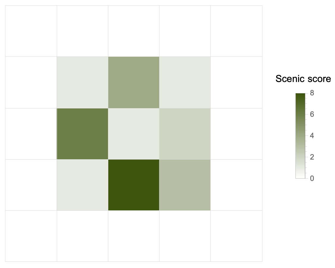
Now things definitely get more complicated, because we have to find the best tree. How? According to a scenic score which is the product of four numbers, one for each side. Each number is the maximum distance along which we can admire the view without being blocked by taller trees.
We must have a function that, given a point (tree) and a list (its row/column “neighbors”), calculates the 4 distances. It increments a counter variable for each lower tree. As soon as it encounters an equal or taller tree, it stops and returns the counter, which will be the distance searched.
counter[value_][list_] :=
 Catch[
  list === {} && Throw[0];
  Block[{total = 0},
   Scan[Which[# < value, ++total, # > value || # == value,
      Throw[++total]] &, list];
   Throw[total]
   ]
  ]
Now we have two steps to get to the solution.
(1) For each point, we find once again the 4 lists of neighboring points (left/right, up/down):
Flatten[MapIndexed[pick[#2, forest] &, forest, {2}], 1]
pick is the middle portion of the VisibleQ function seen in Part 1. I have made it self-contained for simplicity. For instance, for the point (1, 1) of the example input, this function spits out something like: {3, {{}, {0, 3, 7, 3}, {}, {2, 6, 3, 3}}. The point (1, 1) corresponds to the height value 3 and:
- on the left, it has no neighbors (it’s on the left border);
- on the right, it has
{0, 3, 7, 3}, in that exact order; - it has no neighbors above (so it’s in the upper right corner);
- it has
{2, 6, 3, 3}below.
(2) To apply the counter function3 we need a double Map: the first will scroll over lists like {p, {sx, dx, up, down}}. The second will apply counter` to each neighbor list, keeping the reference point fixed. It will come up with another list that will again be a matrix: each point-tree will be associated with the four distances, which, multiplied, will give the scenic score.
All that remains is to find the maximum of this list as a function of the product of the 4 distances. This is easy thanks to MaximalBy:
MaximalBy[
  Map[Map[counter[#[[1]]], #[[2]]] &,
   Flatten[MapIndexed[pick[#2, data] &, data, {2}], 1]],
  Apply[Times]
  ] // Flatten /* Apply[Times]
The last bit, Flatten /* Apply[Times], is just multiplying the resulting 4 values to obtain the scenic score.
😓 It is 23:38 and I have not yet had my evening herbal tea. I’m really starting to believe that I don’t think I will endure until Christmas with this frantic pace of finding the solution and writing the report. I’m going to try, though, as long as I keep up.
Bonus: maps

-
A perfect representation of a field in physics. Inevitable note because the writer is proud of his scientific background, although he likes a lot computer science stuff. ↩︎
-
This is not the right way to slice a 2D list in Python; it’s pseudo-code to give an idea. ↩︎
-
Or at least in the way I wrote it. I thought of simplifying it to allow a clearer application, but I didn’t have time today. I’m sure I’ll go through these notes once again in the future, also because I want to write a Python solution as well. ↩︎
🎄👨💻 Day 7: No Space Left On Device
The dreaded day came, eventually. Without a little hint, I would not have been able to pull out the solution.
The problem was not that I didn’t have a clue on how to solve the puzzle, but that I was stuck with my first approach, refusing to change perspective. That is why the account of this seventh calendar day is perhaps the most important of all the previous ones. Because I found a difficulty that, at first, had completely blocked me. Then a change of point of view allowed me to find the correct solution.
Today’s problem, in short. The Elves’ apparatus has more than its messaging system malfunctioning. You attempt to execute a system update, but it does not go through since there is insufficient disk space available. You inspect the filesystem to examine what’s happening and record the terminal output generated.
The output is very similar to what you would get on a UNIX system. The cd and ls commands are used to change and list the contents of a directory. Each file is associated with its size in bytes (?).
Part 1
Since we have to try to free up space, the first thing to do is to calculate the size of each directory. One directory can contain others, and we have to take this into account to calculate the final size.
My initial idea was to build a data structure that was as similar as possible to the filesystem nested hierarchy. Each entity in this collection of elements had to contain, eventually, other entities (if it were a directory), or simply the name of the file and its size.
I therefore wrote this class:
class Dir:
    """A Dir class"""

    def __init__(self, name):
        self.name = name
        self.children = {}
        self.parent = None
        self.size = 0

    def add(self, child, value=None):
        """Add children to Dir"""
        self.children[child] = value

    def total(self):
        """Total size of this Dir"""
        if self.children:
            for child in self.children.values():
                self.size += child.total() if isinstance(child, Dir) else child
        return self.size

    def __repr__(self):
        return f"Dir({self.children}, parent: '{self.parent.name if self.parent else None}')"
The .total() method already does what one would expect: calculate the total of a directory, following recursively any nested directory. The real stumbling block I haven’t yet overcome was figuring out how to calculate the size of individual directories. Why? Because the puzzle clearly says that, for example, a baz.txt file in the /foo/bar/ directory will contribute to the size of both directories plus the root /. I swear I was unable to write the code that would allow me to do this simple operation.
I was taking too long, so I took a detour on YouTube and was inspired by a video by Jonathan Paulson, a competitive programmer who almost always manages to be in the top 100 people who solve both Advent of Code puzzles. I only had to listen to how he described the problem to figure out how to rewrite the solution. The idea was very simple: simply keep track of each path and its size in a trivial dictionary and without creating a nested object.
Here’s my second attempt with the parsing function:
from collections import defaultdict

def parse(puzzle_input):
    paths = []
    sizes = defaultdict(int)

    for line in puzzle_input.splitlines():
        words = line.strip().split()
        if words[1] == "cd":
            if words[2] == "..":
                paths.pop()
            else:
                paths.append(words[2])
        elif words[1] == "ls" or words[0] == "dir":
            continue
        else:
            size = int(words[0])
            for i in range(1, len(paths) + 1):
                sizes["/".join(paths[:i])] += size

	return sizes
For each line in the input, there are three action we can take:
- Change directory, either down or up. If down, record append the new path to the list of paths. If up, remove the last added path (with our friend
.pop()) - List the content of the directory. We simply ignore this line.
- Read a directory’s content. If a line starts with
dir, it indicates that the current file a directory, so we ignore it: we’re gonna explore that directory later on. If it starts with an integer, we save it.
The following bit of code it’s the interesting one. It’s where we add the size of the current file to all directories it belongs to. That is, to all of its parents up to /. We perform a loop over the parents paths, we build a nice UNIX-like path string, and then add the file size.
size = int(words[0])
for i in range(1, len(paths) + 1):
   sizes["/".join(paths[:i])] += size
Part 1 asks us to find all the directories that are at most 100 000 in size. That’s pretty easy with our sizes dictionary:
def part1(data):
    total = 0
    for size in data.values():
        if size <= 100_000:
            total += size
    return total
Part 2
The second part asks us to find the smallest directory that would allow running the upgrade. We know the total space available and the space required by the update. Thus:
avail = 70_000_000
needed = 30_000_000
max_used = avail - needed
free = data["/"] - max_used
The max_used is the maximum space we are allowed to use. The minimum space we need to free up is the total space we’re occupying, data['/'] – the space of the root directory – minus the allowed maximum. It means two operations: a filtering and then sorting.
def part2(data):
    avail = 70_000_000
    needed = 30_000_000
    max_used = avail - needed
    free = data["/"] - max_used

    candidates = list(filter(lambda s: s >= free, data.values()))

    return sorted(candidates)[0]
Day 7 is done, but I have to thank Jonathan Paulson because, without his hint, I doubt I would have been able to finish today. But that’s what happen when you’re trying to learn, right? You push yourself until it’s not longer easy and you’re stuck with a seemingly insurmountable difficulty. Then, with the help of someone more experienced or by studying the subject a little more, one is often able to overcome the stumbling block. And it is this experience that, as it accumulates, makes all the difference in the world in any learning process.
“Hey, Edoardo, do you have also a nice and elegant solution in the Wolfram Language?”
“Next time, my friend. Perhaps as a Christmas present. Now I’m pretty satisfied with what I got.”
🎄👨💻 Day 6: Tuning Trouble
The preparation phase is finally over, and the expedition in the jungle can begin. You and the Elves set off on foot, each with their backpack filled only with what you’ll need (hopefully). Suddenly, one of the Elves hands you a device. “It has fancy features,” he says, “but you need to set up its communication system right away.” He adds with a grin, ”I heard you know your way around signal-based systems - so this one should be easy for you!” They gave you an old, malfunctioning device that you need to fix. ‘Thanks a lot, friends!’
No sooner had he finished speaking, some sparks signals that the device is partially working! You realize it needs to lock onto their signal. To make it work as it should, you must create a subroutine that detects when four unique characters appear in sequence; this indicates the start of a packet in the communication data-stream.
Your task is clear: given an input buffer, find and report how many characters there are from its beginning to the end of that four-character marker.
Part 1
If we can scan the input and split it in overlapping subsequences of 4 chars, then we could compare them and find the first one that doesn’t contain duplicates characters. That one would be our marker string.
We need to have a utility function for that purpose. It should behave as if a four-characters wide windows scrolled over the string. The offset between one substring and the next is exactly one character. We also need to consider that we might end up with strings that are shorter than the target length if there are not enough characters left.
Here’s our partition() function:
def partition(l, n, d=None, upto=True):
    """
       Generate sublists of `l`
       with length up to `n` and offset `d`
    """
    offset = d or n
    return [
        lx for i in range(0, len(l), offset)
        if upto or len(lx := l[i : i + n]) == n
    ]
To obtain the solution, we need to transform each sublist into a set to remove any duplicates. Only the resulting sets whose length is still 4 characters are potential candidates for our marker string. We can filter out the others and take the first one. Then, find the index in the original string where our substring starts. Python has the str.find(substr) method for that precise purpose.
def part1(data):
    pdata = list(map(set, partition(data, n=4, d=1, upto=False)))
    marker = list(filter(lambda x: len(x) == 4, pdata))[0]
    return ("".join(data)).find("".join(marker)) + 4
Why are we summing 4 at the end? Because the puzzle asks for “the number of characters from the beginning of the buffer to the end of the first such four-character marker.”
Part 2
There’s a slight plot twist: we also need to decode the start of messages with another, appropriate marker. This time, the marker string is 14 characters long. Once again, our partition() function is versatile enough: we only need to change the offset argument to 14. The code is identical to Part 1’s.
My source of inspiration
As I was able to find the complete solution in a short time, I took some time to make some comparisons with another programming language. A particularly special language since it was the first one I learned: the Wolfram Language (now “WL” for short). For this kind of tasks, it really excels, I have to say. The idea of implementing the partition() function came from remembering that WL has an identical function with many, many more options.
The elegance of the solution written in WL is astonishing (but, as I said, I’m completely biased). I let the reader judge by themselves.
With[{sample = inputDay6},
 Flatten/*Last@
  StringPosition[sample,
   StringJoin@Select[
     Partition[Characters@sample, 4, 1],
     DuplicateFreeQ, 1]
   ]
 ]
🎄👨💻 Day 5: Supply Stacks
It’s starting to get serious today, at least as far as input parsing is concerned. The Elves are still in the process of unloading the materials needed for the expedition. On the cargo ship, the material is arranged in crates stacked in a certain order. It would be too easy (and unrealistic) if we could unload all the crates. The ones we need are scattered on the ship, piled in different groups.
The ship’s operator is quick to determining in what order to move the crates so as to retrieve those that the Elves need. They, however, forgetful as they are, do not remember which crates will be the ones they can unload first, that is, the ones that will be at the top of each stack at the end of the “sorting” procedure.
Part 1
The input is divided into two parts. The first, the different stacks with crates before the intervention of the operator. The second, the list of rearrangement operations. It is the first part that is problematic. The example input reads
    [D]
[N] [C]
[Z] [M] [P]
1   2   3
If the operator were to move 2 crates from the second to the third stack, for example, she will move one at a time. Which means that the order of the crates will be reversed: the first crate moved will end up as far back as possible in the stack to which it is moved.
In order to handle crate stacks as if they were lists, we need to find a way to convert a list like [[D], [N,C], [Z,M,P]] to [[Z,N], [M,C,D], [P]]. Unfortunately, this is not a simple transposition, but two operations are needed:
-
Reverse the matrix, that is, read it row-by-row from the bottom
-
Now transpose the matrix
For the two steps to work, one more thing is necessary: you must keep the blanks. For example, the first line cannot be [ [D] ], but must be [ [blank, D, blank] ].
There is another problem to handle in parsing the input if we want the transpose operation to make sense: the array must be square, or at least rectangular.
The steps to parse the input are the following:
-
Split the stacks initial configuration from the rearrangement procedure (easy: it’s just a double
\n\n) -
Save how many columns we have, that’s important. It can be done by counting the number of digits at the very bottom of the stacks configuration
-
Read the list of moves. I used the regular expression
r"move (\d+) from (\d) to (\d)"to read in a tuple like(num, src, dest):numis how many crates are moved,srcfrom which stack anddestto which one
And now, the fun part. To process the stacks configuration and obtain our matrix, we need to:
-
Read each line of the stacks section and strip any non-letter character. We also replace any empty “slot” with a dot (
.) placeholder, needed to have a square, transposable matrix -
If the number of
rowsis less than the number ofcols, we need to add extra rows (filled with dots). Again, that’s to obtain a square matrix. How many rows? Enough to haverows == cols, that is,["." * cols] * (cols - rows) -
Now we can transform our matrix. We reverse it first, and then transpose rows and columns
-
Last step: we get rid of all the dot placeholders, which represent non-existent crates (or empty ones, if you want). This can be done with
filter(lambda x: x != ".", stack)
I’m 99% sure that’s not the easiest or clearest way, but I had so much fun in trying to implement this matrix approach1. The problem resembles a lot the Hanoi Towers’ puzzle, and I bet there are hundreds of schemes or algorithms to solve it.
To obtain the answer to Part 1, we only need to process our stacks according to the list of moves. Remember: we must move the crates one by one. That’s easy enough now that we have our matrix of stacks:
def part1(data):
    stacks, moves = data
    for num, src, dest in moves:
        s, d, n = int(src) - 1, int(dest) - 1, int(num)
        for _ in range(n):
            stacks[d].append(stacks[s].pop())
    return "".join(map(lambda x: x[-1], stacks))
We also need to decrement all the indexes in each move because Python counts from zero. The return statement simply takes the topmost crate in each stack and then joins the characters to get the final answer 🎉.
Part 2
It has to be expected: it turns out that the “giant cargo crane” can move more than one crate at a time. Even better: as many as we want. The code change is minimal because the bulk of the work was reading and saving the crates stack in the right way.
The only thing that changes is that we don’t need the loop for _ in range(n) because we can move more than one crate at a time. We also cannot use pop() because it does not support a range, so we have to do it by hand: extract the elements we are interested in and then delete them.
def part2(data):
    stacks, moves = data
    for num, src, dest in moves:
        s, d, n = int(src) - 1, int(dest) - 1, int(num)
        stacks[d].extend(stacks[s][-n:])
        del stacks[s][-n:]
    return "".join(map(lambda x: x[-1], stacks))
It's 11:59 pm, and Day 5 is finally over. Unexpectedly tough.
🎄👨💻 Day 4: Camp Cleanup
Today the Elves start working for real: they need to clear the base camp to make enough space to unload the rest of the material for the upcoming expedition.
“Let’s divide the whole area to clear,” an Elf suggests.
“Good idea, let me take care of it,” another one replies.
So the enthusiastic Elf divides the sections and assigns them to the other Elves who will work in pairs. Each pair will work on two ranges of sections, for example 2,4-6,8: the first Elf will handle sections 2 to 4, the second from 6 to 8.
Unfortunately, the enthusiastic Elf made a bit of a mess. He didn’t realize he assigned overlapping ranges. So we have to find out how many sections are already contained in others, so that we can reassign them and avoid unnecessary work for the Elves.
Part 1
As on Day 3, the anatomy of the problem suggests using sets. We need to determine if a group of numbers is a subset of another or which numbers two groups have in common. Both of these operations are immediate with a set.
Perhaps the most interesting part of today’s puzzle is how to parse the input. We have:
2-4,6-8
2-3,4-5
5-7,7-9
...
and we want
[
 [[2,4], [6,8]],
 [[2,3], [4,5]],
 [[5,7], [7,9]],
 ...
]
We can do the first step of input parsing in one line (because it’s fun):
data = [
 list(map(lambda p: list(map(int, p.split("-"))), pair.split(",")))
 for pair in puzzle_input.splitlines()
]
- We split each line at
, - Each of the elements of this list is split again at
-, and then each element is converted to integer withmapand thelambdafunction.
The second step of the parsing phase is to build a “list of pairs of sets”, where each element of the pair includes all the IDs in the range. Here we need to consider one important detail: the ranges must include the last ID. Hence, we must increment by 1 the second element of each range, otherwise Python will ignore it. That’s a for loop and another map:
sets = []
for p1, p2 in data:
	# range must be inclusive
	p1[1] += 1
	p2[1] += 1
	p1, p2 = map(lambda x: set(range(*x)), (p1, p2))
	sets.append((p1, p2))
Once we did that, the solution to Part 1 is almost immediate: we only need to find if, in each pair, any set is a subset of the other, and count how many of these overlapping sets there are:
def part1(data):
    overlaps = 0
    for p1, p2 in data:
        if p1 <= p2 or p1 >= p2:
            overlaps += 1
    return overlaps
Part 2
The second part of the problem asks us to find (and count) those pairs of ID ranges that overlap for at least one ID. The total will necessarily be greater than the number found in Part 1. The way we read the input allows us to find the solution by changing only one line from Part 1:
def part2(data):
    overlaps = 0
    for p1, p2 in data:
        if p1 & p2:
            overlaps += 1
    return overlaps